Project Overview
In this project, I employ several supervised algorithms to accurately predict an individual income using data collected from the 1994 U.S. Census.
We implement various testing procecures to choose the best candidate algorithm from preliminary results and further optimize this algorithm to best model the data.
The primary goal of this implementation is to construct a model that accurately predicts whether an individual makes more than $50,000. This sort of task can arise in a non-profit setting, where organizations survive on donations.
Understanding an individual's income can help a non-profit better understand how large of a donation to request, or whether or not they should reach out to begin with. While it can be difficult to determine an individual's general income bracket directly from public sources, we can infer this value from other publically available features.
This project was submitted as part of the requisites required to obtain Machine Learning Engineer Nanodegree from Udacity.
Dataset
The dataset for this project originates from the UCI Machine Learning Repository.
The datset was donated by Ron Kohavi and Barry Becker, after being published in the article "Scaling Up the Accuracy of Naive-Bayes Classifiers: A Decision-Tree Hybrid". Article by Ron Kohavi online.
The data we investigate here consists of small changes to the original dataset, such as removing the 'fnlwgt' feature and records with missing or ill-formatted entries.
Exploring the Data
We the code cell below to load necessary Python libraries and load the census data.
The last column from this dataset, 'income', will be our target label (whether an individual makes more than, or at most, $50,000 annually). All other columns are features about each individual in the census database.
# Import libraries necessary for this project
import numpy as np
import pandas as pd
from time import time
from IPython.display import display # Allows the use of display() for DataFrames

# Import supplementary visualization code visuals.py
import visuals as vs

# Pretty display for notebooks
%matplotlib inline

# Load the Census dataset
data = pd.read_csv("census.csv")

# Success - Display the first five records
display(data.head(n=5))
Implementation: Data Exploration
A cursory investigation of the dataset determines how many individuals fit into either group, and will tell us about the percentage of these individuals making more than \$50,000.
In the code cell below, we compute the following:
- The total number of records,
'n_records' - The number of individuals making more than \$50,000 annually,
'n_greater_50k'. - The number of individuals making at most \$50,000 annually,
'n_at_most_50k'. - The percentage of individuals making more than \$50,000 annually,
'greater_percent'.
# TODO: Total number of records
n_records = data.income.count()

# TODO: Number of records where individual's income is more than $50,000
n_greater_50k = data[data.income==">50K"].income.count()

# TODO: Number of records where individual's income is at most $50,000
n_at_most_50k = data[data.income=="<=50K"].income.count()

# TODO: Percentage of individuals whose income is more than $50,000
greater_percent = 100.0 * n_greater_50k/n_records

# Print the results
print "Total number of records: {}".format(n_records)
print "Individuals making more than $50,000: {}".format(n_greater_50k)
print "Individuals making at most $50,000: {}".format(n_at_most_50k)
print "Percentage of individuals making more than $50,000: {:.2f}%".format(greater_percent)
Feature Characteristics
- age: continuous.
- workclass: Private, Self-emp-not-inc, Self-emp-inc, Federal-gov, Local-gov, State-gov, Without-pay, Never-worked.
- education: Bachelors, Some-college, 11th, HS-grad, Prof-school, Assoc-acdm, Assoc-voc, 9th, 7th-8th, 12th, Masters, 1st-4th, 10th, Doctorate, 5th-6th, Preschool.
- education-num: continuous.
- marital-status: Married-civ-spouse, Divorced, Never-married, Separated, Widowed, Married-spouse-absent, Married-AF-spouse.
- occupation: Tech-support, Craft-repair, Other-service, Sales, Exec-managerial, Prof-specialty, Handlers-cleaners, Machine-op-inspct, Adm-clerical, Farming-fishing, Transport-moving, Priv-house-serv, Protective-serv, Armed-Forces.
- relationship: Wife, Own-child, Husband, Not-in-family, Other-relative, Unmarried.
- race: Black, White, Asian-Pac-Islander, Amer-Indian-Eskimo, Other.
- sex: Female, Male.
- capital-gain: continuous.
- capital-loss: continuous.
- hours-per-week: continuous.
- native-country: United-States, Cambodia, England, Puerto-Rico, Canada, Germany, Outlying-US(Guam-USVI-etc), India, Japan, Greece, South, China, Cuba, Iran, Honduras, Philippines, Italy, Poland, Jamaica, Vietnam, Mexico, Portugal, Ireland, France, Dominican-Republic, Laos, Ecuador, Taiwan, Haiti, Columbia, Hungary, Guatemala, Nicaragua, Scotland, Thailand, Yugoslavia, El-Salvador, Trinadad&Tobago, Peru, Hong, Holand-Netherlands.
Data Preprocessing.
Before the dataset can be used as input for machine learning algorithms, we clean, format, and restructure it.
In this dataset there are no invalid or missing entries, however, there are some qualities about certain features that must be adjusted to enhance the redictive power of the implemented machine learning models.
Transforming Skewed Continuous Features
In the following we investigage whether the dataset contains at least one feature whose values tend to lie near a single number, or whose values have a non-trivial number of vastly larger or smaller values than that single number. Such distributions of values can make the learning algorithms to underperform if the range is not properly normalized.
This step is neccessary to reduce potential unstabilities of the algorithms used below.
With the census dataset two features fit this description: 'capital-gain' and 'capital-loss'.
We run the code cell below to plot a histogram of these two features.
# Split the data into features and target label
income_raw = data['income']
features_raw = data.drop('income', axis = 1)

# Visualize skewed continuous features of original data
vs.distribution(data)

For highly-skewed feature distributions such as 'capital-gain' and 'capital-loss', it is common practice to apply a logarithmic transformation on the data so that the very large and very small values do not negatively affect the performance of the learning algorithms.
Using a logarithmic transformation will significantly reduce the range of values caused by outliers.
Since the logarithm of 0 is undefined, we translate the values by a small amount above 0 to apply the the logarithm successfully.
We run code cell below to perform a transformation on the data and visualize the results.
# Log-transform the skewed features
skewed = ['capital-gain', 'capital-loss']
features_log_transformed = pd.DataFrame(data = features_raw)
features_log_transformed[skewed] = features_raw[skewed].apply(lambda x: np.log(x + 1))

# Visualize the new log distributions
vs.distribution(features_log_transformed, transformed = True)

Normalizing Numerical Features
In addition to performing transformations on features that are highly skewed, we also scale the numerical features.
Below, we implement a normalization procedure to ensure that each feature is treated equally when applying supervised learning algorithms. The scaling applied to the data does not change the shape of each feature's distribution
Note: once scaling is applied, observing the data in its raw form will no longer have the same original meaning, see below.
We run the code cell below to normalize each numerical feature. We use sklearn.preprocessing.MinMaxScaler.
# Import sklearn.preprocessing.StandardScaler
from sklearn.preprocessing import MinMaxScaler

# Initialize a scaler, then apply it to the features
scaler = MinMaxScaler() # default=(0, 1)
numerical = ['age', 'education-num', 'capital-gain', 'capital-loss', 'hours-per-week']

features_log_minmax_transform = pd.DataFrame(data = features_log_transformed)
features_log_minmax_transform[numerical] = scaler.fit_transform(features_log_transformed[numerical])

# Show an example of a record with scaling applied
display(features_log_minmax_transform.head(n = 5))
Data Preprocessing
The table above contains several features for each record that are categorical (non-numeric).
Below we convert categorical variables by using a one-hot encoding procedure. This encoding creates a "dummy" variable for each possible category of each non-numeric feature.
Additionally, as with the non-numeric features, we need to convert the non-numeric target label, 'income' to numerical values for the learning algorithm to work.
Since there are only two possible categories for this label ("<=50K" and ">50K"), we can avoid using one-hot encoding and simply encode these two categories as 0 and 1, respectively.
In code cell below, we implement the following:
- We use
pandas.get_dummies()to perform one-hot encoding on the'features_raw'data.
- We convert the target label
'income_raw'to numerical entries.- Set records with "<=50K" to
0and records with ">50K" to1.
- Set records with "<=50K" to
# TODO: One-hot encode the 'features_log_minmax_transform' data using pandas.get_dummies()
features_final = pd.get_dummies(features_log_minmax_transform)

# TODO: Encode the 'income_raw' data to numerical values
def nEnc(x):
    if x =='>50K': return 1
    else: return 0
income = income_raw.apply(nEnc)

# Print the number of features after one-hot encoding
encoded = list(features_final.columns)
print "{} total features after one-hot encoding.".format(len(encoded))

# Uncomment the following line to see the encoded feature names
#print encoded
Splitting the Data into Training and Test Sets
Now that all categorical variables have been converted into numerical features, and all numerical features have been normalized, we can proceed to split the dataset into training and test sets.
Below, 80% of the data will be used for training and 20% for testing.
We run the code cell below to perform this split:
# Import train_test_split
from sklearn.cross_validation import train_test_split

# Split the 'features' and 'income' data into training and testing sets
X_train, X_test, y_train, y_test = train_test_split(features_final,
                                                    income,
                                                    test_size = 0.2,
                                                    random_state = 0)

# Show the results of the split
print "Training set has {} samples.".format(X_train.shape[0])
print "Testing set has {} samples.".format(X_test.shape[0])
Evaluating Model Performance
In this section, we investigate four different supervised learning algorithms, and determine which is best at modeling the data.
Problem Statement
Metrics and the Naive Predictor
A charity organization, "CharityML", equipped with their research, knows individuals that make more than \$50,000 are most likely to donate to their charity. Because of this, *CharityML* is particularly interested in predicting who makes more than \$50,000 accurately.
It would seem that using accuracy as a metric for evaluating model performace would be appropriate. Additionally, identifying someone that does not make more than \$50,000 as someone who does would be detrimental to CharityML, since they are looking to find individuals willing to donate.
In the present context, a precise prediction of those individuals that make more than \$50,000 is more important than to recall those individuals.
Given the above, we can use F-beta score as a metric that considers both precision and recall. The F-beta score is defined as follows,
$$ F_{\beta} = (1 + \beta^2) \cdot \frac{precision \cdot recall}{\left( \beta^2 \cdot precision \right) + recall} $$In particular, when $\beta = 0.5$, more emphasis is placed on precision. This is called the F$_{0.5}$ score (or F-score for simplicity).
Looking at the distribution of classes (those who make at most \$50,000, and those who make more), it's clear most individuals do not make more than \$50,000. This can greatly affect accuracy, since we could simply say "this person does not make more than \$50,000" and generally be right, without ever looking at the data!
Making the above a statement would be called naive, since we have not considered any information to substantiate the claim.
In our modeling, we also consider the naive prediction for the data, to help establish a benchmark for whether a particular model is performing well. That been said, using that prediction would be pointless: If we predicted all people made less than \$50,000, CharityML would identify no one as donors.
Metric definitions:
Accuracy
Measures how often the classifier makes the correct prediction. It’s the ratio of the number of correct predictions to the total number of predictions (the number of test data points).
Precision
It is a ratio of true positives to all positives, in other words it is the ratio of
[True Positives/(True Positives + False Positives)]
Recall or Sensitivity
It is a ratio of true positives to all the words that were actually spam, in other words it is the ratio of
[True Positives/(True Positives + False Negatives)]
Remarks
Our classification problem is skewed in the classification distributions, therefore accuracy by itself is not a very good performance metric. In our case, precision and recall can be combined to get the F1 score, which is weighted average of the precision and recall scores.
The F1 score can range from 0 to 1, with 1 being the best possible score (we take the harmonic mean as we are dealing with ratios).
Naive Predictor Performace
In the following we implement a naive predictor model that always predicts an individual making more than $50,000. We want to find this model's accuracy and F-score when trained in our dataset.
We use the code cell below and assign the results to 'accuracy' and 'fscore' to be used later.
'''
TP = np.sum(income) # Counting the ones as this is the naive case. Note that 'income' is the 'income_raw' data
encoded to numerical values done in the data preprocessing step.
FP = income.count() - TP # Specific to the naive case

TN = 0 # No predicted negatives in the naive case
FN = 0 # No predicted negatives in the naive case
'''
# TODO: Calculate accuracy, precision and recall
TP = float(np.sum(income))
FP = float(income.count()-TP)
TN=0.0
FN=0.0
beta = 0.5

accuracy = (TP + TN)/(FP+FN+TP+TN)
recall = TP/(TP+FN)
precision = TP/(TP+FP)

# TODO: Calculate F-score using the formula above for beta = 0.5 and correct values for precision and recall.
# HINT: The formula above can be written as (1 + beta**2) * (precision * recall) / ((beta**2 * precision) + recall)
fscore =  (1.0 + beta**2) * (precision * recall) / ((beta**2 * precision) + recall)

# Print the results
print "Naive Predictor: [Accuracy score: {:.4f}, F-score: {:.4f}]".format(accuracy, fscore)
Naive predictor results:
The results of running the cell code above are:
Naive Predictor accuracy score: 0.2478 Naive Predictor F-score: 0.2917
Supervised Learning Models
The following are some of the supervised learning models that are currently available in scikit-learn, which we implement in the following sections.
- Gaussian Naive Bayes (GaussianNB)
- Decision Trees
- Ensemble Methods (Bagging, AdaBoost, Random Forest, Gradient Boosting)
- K-Nearest Neighbors (KNeighbors)
- Stochastic Gradient Descent Classifier (SGDC)
- Support Vector Machines (SVM)
- Logistic Regression
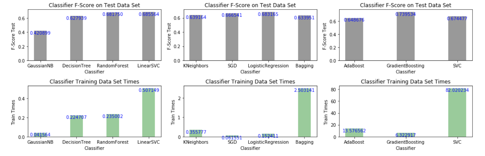
Out of the algorithms listed above, we aim to use three supervised learning models to carry out our data analysis. To this end, I generated a collection of bar graphs indicating the value of the performance metric (f-score) together with the algorithm training time.
I selected three classifiers yielding the highest f-score and reasonably short training times. Amongst the slow algorithms (righ-panel), Gradient Boosting yielded the highest f-score of all classifiers tested; among the intermediate algorithms (middle panel) logistic regression runs fast and yields the best score in that group. In the left panel, linear supporve vector machine (SVC) yields the hightes f-score; Random Forest is a good choice as well.
The figure below displays the results (the benchmarking code appears after the next discussion).
Algorithm Characteristics:
1. Gradient Boosting:
*1.1 Application:
- It is a popular approach to ensemble learning for applications in which real-time performance is required, such as face detection systems capable of detecting faces in real-time with both high detection rate and very low false positive rates.
*1.2 Strengths:
The goal of gradient boosting is to boost the performance of a linear combination of weak learning algorithms.
A gradient boost classifier learns from the mistakes of the previous weak learners in the ensemble and only selects those features known to improve the predictive power of the model.
It is a generalization of the AdaBoost algorithm. It uses gradients (gradient descent) instead of re-weighting to boost the shortcomings of misclassified labels.
It can be used for regression, classification and raking.
It is able to handle a variety of loss functions.
Execution times can be handled appropriately and improved in proportion to available computational resources.
*1.3 Weaknesses:
Making weak classifiers too complex can lead to overfitting.
Making weak classifiers too weak can lead to low margins, which can also result in overfitting.
Boosting very complex underlying learner algorithms that intrinsically overfit the model will lead to an overfitted results; oftentimes this also can lead to convergence issues.
*1.4 Appropriateness:
Boosting can be really successful in boosting algorithms developed for binary classification. As discussed in the data preprocessing section, the training dataset contains imbalanced classes and constitutes essentially a binary classification problem.
Gradient boosting can handle class imbalance by constructing successive training sets based on incorrectly classified examples.
As we are dealing with imbalanced data, we need to be cautiuos and monitor whether the algorithm predicts all the cases into majority classes without loss of overall accuracy.
2.- Logistic Regression:
*2.1 Application:
It is perhaps arguably the most popular method for binary classification problems. A common application is in the field of financial risk analysis where LR can be applied to predict the risk of customer defaulting on their debts scheduled payments or the probability of a banking transaction to be fraudulent.
*2.2 Strengths:
- Easy to implement and very efficient to train.
- Serves as a good benchmark before exploring more complex algorithms.
- Imbalances in the training datasets affect only the estimate of the model intercept.
*2.3 Weaknesses:
- As is, it is restricted to linear problems.
- Hypothesis space is limited.
- Imbalances in the training dataset can results in the skewing of the predicted probabilities.
*2.4 Appropriateness:
- Our problem can be casted as binary classification problem and as such, logistic regression can work as a good prototype to benchmark the model. Potential imbalances in the data set may be alleviated using cross validation and designing appropriate thresholding criterions to make predictions.
3.- Support Vector Machines:
*3.1 Application:
Support vector machines are widely applied in both classification and regression problems. In bioinformatics, these methods are applied in protein and gene expression classification. Likewise, they are applied in clinical biostatistics in the design of disease (e.g. cancer) detection protocols.
*3.2 Strengths:
In particular, linear support vector machines are naturally fitted to solve binary classification problems as the classifier is a separating hyperplane.
Capable of handling very large feature spaces, i.e. complexity is weakly dependent on the dimensionality of feature space.
Model simplification is facilitated by feature selection, which can result in shorter training times and better convergence.
Overfitting can be reasonably controlled by the soft margin approach
*3.3 Weaknesses:
Better suited for binary classification; multiclass classification requires reducing the multiclass problem into multiple binary classification problems.
Requires full labeling of input data; parameters of resulting model are sometimes difficult to interpret.
Susceptible to noise, i.e. uncontrolled mislabeled examples can dramatically decrease performance.
*3.4 Appropriateness:
- For our particular binary classification problem, the linear SVM is capable of finding the optimal separating hyperplane for imbalanced classes. With default settings, in addition to yielding a better f-score, the Linear SVM is orders of magnitude faster than SVM as seen in our bar charts above.
Benchmarking - Training/Testing Pipeline on a Fixed Sample Size
To properly evaluate the performance of each model, we create a training and predicting pipeline that allows to quickly and effectively train models using various sizes of training data and perform predictions on the testing data.
In the cell code below we implement this pipeline using a fixed sample size. In a later section, we employ different sample sizes.
#The code below generates bar chart plots of f-scores and elapsed time for training datasets
#It aims to guide the selection of three classifiers to be discussed
#*** makes use of train_predict function defined in cell In [10]
#Juan E. Rolon

import matplotlib.pyplot as plt
from sklearn.naive_bayes import GaussianNB
from sklearn import linear_model
from sklearn.metrics import fbeta_score
from sklearn.metrics import accuracy_score
from sklearn.tree import DecisionTreeClassifier
from sklearn.ensemble import RandomForestClassifier
from sklearn.svm import LinearSVC
from sklearn.svm import SVC
from sklearn.ensemble import AdaBoostClassifier
from sklearn.ensemble import GradientBoostingClassifier
from sklearn.ensemble import BaggingClassifier
from sklearn.linear_model import SGDClassifier
from sklearn.neighbors import KNeighborsClassifier
from sklearn.linear_model import LogisticRegression

#Instantiate classifier objects and stored them in a list for later access

gnb = GaussianNB()
dt = DecisionTreeClassifier(random_state=0)
bags = BaggingClassifier(KNeighborsClassifier(), random_state=10, n_jobs=6)
bdt = AdaBoostClassifier(DecisionTreeClassifier(random_state=20), algorithm="SAMME")
rfc = RandomForestClassifier(random_state=90, n_jobs=6)
gdb = GradientBoostingClassifier(random_state=30)
knn = KNeighborsClassifier(n_jobs=6)
stgd = SGDClassifier(random_state=40, n_jobs=6)
lsvc = LinearSVC(random_state=80)
svc = SVC(random_state=60)
lreg = LogisticRegression(random_state=50)

clf_list = [[gnb, dt, rfc, lsvc], [knn, stgd, lreg, bags], [bdt, gdb, svc]]

#Create lists to store selected benchmarking results
clf_lscores = []
clf_ltrain_times = []
clf_lnames = []

#Train all classifiers on training data and make predictions on test data
#Store desired benchmarking results
for j in range(len(clf_list)):
    temp_scores = []
    temp_times = []
    temp_names = []
    for i in range(len(clf_list[j])):
        clf_results = train_predict(clf_list[j][i], len(y_train), X_train, y_train, X_test, y_test)
        temp_scores.append(clf_results['f_test'])
        temp_times.append(clf_results['train_time'])
        temp_names.append(clf_results['clf_name'].replace('Classifier', ''))
    clf_lscores.append(temp_scores)
    clf_ltrain_times.append(temp_times)
    clf_lnames.append(temp_names)

print clf_lnames
print clf_lscores
print clf_ltrain_times

#Generate bar chart plots using selected benchmarking results

plt.figure(1, figsize=(15, 5))

for j in range(len(clf_lscores)):

    n_groups = len(clf_lscores[j])
    index = np.arange(n_groups)
    bar_width = 0.35
    opacity = 0.4
    impdata1 = clf_lscores[j]
    impdata2 = clf_ltrain_times[j]
    plt.subplot(2, 3, j+1)
    plt.xlabel('Classifier')
    plt.ylabel('F-Score Test ')
    plt.title('Classifier F-Score on Test Data Set')
    plt.xticks(index, clf_lnames[j])
    bar1 = plt.bar(index, impdata1, bar_width, alpha=opacity, color='k')
    for rect in bar1:
        height = rect.get_height()
        plt.text(rect.get_x() + rect.get_width()/2.0, height, '%f' % height, ha='center', va='top',color='b')
    plt.subplot(2, 3, j+4)
    plt.xlabel('Classifier')
    plt.ylabel('Train Times ')
    plt.title('Classifier Training Data Set Times')
    plt.xticks(index, clf_lnames[j])
    bar2 = plt.bar(index, impdata2, bar_width, alpha=opacity, color='g')

    for rect in bar2:
        height = rect.get_height()
        plt.text(rect.get_x() + rect.get_width()/2.0, height, '%f' % height, ha='center', va='top',color='b')

plt.tight_layout()
plt.show()

Creating a Training and Predicting Pipeline for Different Sample Sizes
In the following we train different models using various sizes of training data and perform predictions on the testing data.
In the code block below, we implement the following:
- Import
fbeta_scoreandaccuracy_scorefromsklearn.metrics.
- We fit the learner to the sampled training data and record the training time.
- We perform predictions on the test data
X_test, and also on the first 300 training pointsX_train[:300].- Record the total prediction time.
- We calculate the accuracy score for both the training subset and testing set.
- We alculate the F-score for both the training subset and testing set.
# TODO: Import two metrics from sklearn - fbeta_score and accuracy_score
# DONE
from sklearn.metrics import fbeta_score
from sklearn.metrics import accuracy_score

def train_predict(learner, sample_size, X_train, y_train, X_test, y_test):
    '''
    inputs:
       - learner: the learning algorithm to be trained and predicted on
       - sample_size: the size of samples (number) to be drawn from training set
       - X_train: features training set
       - y_train: income training set
       - X_test: features testing set
       - y_test: income testing set
    '''

    results = {}

    # TODO: Fit the learner to the training data using slicing with 'sample_size' using .fit(training_features[:], training_labels[:])

    start = time() # Get start time
    learner = learner = learner.fit(X_train[:sample_size],y_train[:sample_size])
    end = time() # Get end time

    # TODO: Calculate the training time

    results['train_time'] = end-start

    # TODO: Get the predictions on the test set(X_test),
    #       then get predictions on the first 300 training samples(X_train) using .predict()

    start = time() # Get start time
    predictions_test = learner.predict(X_test)
    predictions_train = learner.predict(X_train[:300])
    end = time() # Get end time

    # TODO: Calculate the total prediction timeE
    results['pred_time'] = end-start

    # TODO: Compute accuracy on the first 300 training samples which is y_train[:300]
    results['acc_train'] = accuracy_score(y_train[:300], predictions_train)

    # TODO: Compute accuracy on test set using accuracy_score()
    results['acc_test'] = accuracy_score(y_test, predictions_test)

    # TODO: Compute F-score on the the first 300 training samples using fbeta_score()
    results['f_train'] = fbeta_score(y_train[:300], predictions_train, beta=0.5)

    # TODO: Compute F-score on the test set which is y_test
    results['f_test'] = fbeta_score(y_test, predictions_test, beta=0.5)

    # Success
    print "{} trained on {} samples.".format(learner.__class__.__name__, sample_size)

    # Added two additional key:values << Juan E. Rolon
    # -------------------------------------------------
    results['clf_name'] = learner.__class__.__name__
    results['samp_size'] = sample_size
    #-------------------------------------------------

    # Return the results
    return results
Initial Model Evaluation
In the code cell, we implement the following:
Import the three supervised learning models discussed in the previous section.
Initialize the three models and store them in
'clf_A','clf_B', and'clf_C'.- Use a
'random_state'for each model used, if provided. - Note: Use the default settings for each model — tune one specific model in a later section.
- Use a
- Calculate the number of records equal to 1%, 10%, and 100% of the training data.
- Store those values in
'samples_1','samples_10', and'samples_100'respectively.
- Store those values in
# TODO: Import the three supervised learning models from sklearn

from sklearn.svm import LinearSVC
from sklearn.ensemble import GradientBoostingClassifier
from sklearn.linear_model import LogisticRegression


# TODO: Initialize the three models

gdb = GradientBoostingClassifier(random_state=30)
lsvc = LinearSVC(random_state=80)
lreg = LogisticRegression(random_state=50)

# TODO: Calculate the number of samples for 1%, 10%, and 100% of the training data
# HINT: samples_100 is the entire training set i.e. len(y_train)
# HINT: samples_10 is 10% of samples_100
# HINT: samples_1 is 1% of samples_100
samples_100 = int(len(y_train))
samples_10 = int(0.1*samples_100)
samples_1 = int(0.01*samples_100)

# Collect results on the learners
results = {}
for clf in [gdb, lsvc, lreg]:
    clf_name = clf.__class__.__name__
    results[clf_name] = {}
    for i, samples in enumerate([samples_1, samples_10, samples_100]):
        results[clf_name][i] = \
        train_predict(clf, samples, X_train, y_train, X_test, y_test)

# Run metrics visualization for the three supervised learning models chosen
vs.evaluate(results, accuracy, fscore)

Improving Training Results by Gridsearch Optimization
Our strategy to improve the learning results consists of the following:
- We choose from the three supervised learning models the best model.
- We then perform a grid search optimization for the model over the entire training set (
X_trainandy_train) by tuning at least one parameter to improve upon the untuned model's F-score.
Now, based on the evaluation we performed earlier, we want to explain to CharityML which of the three chosen models is the most appropriate for the task of identifying individuals that make more than \$50,000.
To this end, we report and discuss the following:
- metrics - F score on the testing when 100% of the training data is used,
- prediction/training time
- the algorithm's suitability for the data.
Optimal Model
According to the results, GradientBoosting appears to be the most appropriate model for the task at hand.
Gradient boosting
This algorithm belongs to the class of machine learning algorithms called boosting ensemble methods. The idea of these methods is to combine several weak learners (ensemble of predictors or classifier algorithms) to form a strong learner during the training process. By weak learner we meant to say an algorithm whose performance metrics are poor, i.e. it does slightly better than random guessing when classifying examples. In particular, gradient boosting works by sequentially adding new predictors to the ensemble, each correcting the predictions of its predecessor. However, instead of tweaking the example instances weights at every iteration, gradient boosting fits the new predictor to the residual errors made by the previous predictor; here the residual errors are interpreted as the absolute value of the difference between the predicted labels and the actual values of the labels provided in the training set.
We can illustrate the entire process as follows. We initially train a non-optimized classifier that we assume to be weak. This classifier will output a set of classification predictions on the given examples on the training dataset. Based on the residual errors made by the first predictor, we train a second classifier of the same type; and again, based on the residual errors made by this second classifier on making a new set of prediction, we train a third classifier and so on. The residual errors are proportional to the rate of change or gradient of some "loss function", which basically represents the price paid for the inaccuracy of predictions. Therefore, the idea is to minimize this loss, and gradient boosting does this minimization by "moving" in sample or feature space in the opposite direction of the gradient, hence the name of the method.
References:
Zhi-Hua Zhou, Ensemble Methods Foundations and Algorithms, CRC Press (2012).
Gradient Boosting. https://en.wikipedia.org/wiki/Gradient_boosting
Factors Involved in the Selection of Gradient Boosting as the Optimal Model
There are several factors that were considered for this selection:
- Firstly, we want our model to precisely predict individuals that make more than 50,000 dlls. from a population sample where most of the individuals make less than this amount. In other words, we want to achieve the best performance metrics for our model, taking into account potential imbalances in the dataset. These imbalances result from the skewing of these two class distributions. Based on this, is not enough to weigh only on classification accuracy, but also on a performace metric such as the f-beta score. It is clear from the bar plots above that GradientBoosting achieves both the highest accuracy and f-beta score among the classifiers when testing the model on the entire dataset.
- Secondly, our model should rely on an algorithm that deals appropriately with potential data imbalances. Indeed, one of the strenghts of GradientBoosting is its ability to handle class imbalances by constructing successive training sets based on incorrectly classified examples (identifying someone that does not make more than 50,000 dlls. as someone who does).
- Lastly, we should look for a model whose computational overhead or runtime scales-up reasonably with the size of the training dataset, without compromising the performance metrics. Although gradient boosting seems to be 1 to 4 orders of magnitude slower than LinearSVM and Logistic Regression, it yields an appreciable higher f-beta score. We believe that runtime can be handled appropiately by our in-house HPC cluster or by purchasing on-demand access to services such as Amazon HPC or Amazon ML, if needed.
Tuning and Optimizing Gradient Boosting
To enhance the predictive power of our chose learning algorith, we use grid search (GridSearchCV) with at least one important parameter tuned with at least 3 different values. We use the entire training set in this step.
In the code cell below, we implement the following:
- Initialize the classifier chosen and store it in
clf.- Set a
random_stateif one is available to the same state set before.
- Set a
- Create a dictionary of parameters aimed for tuning for the chosen model.
- Example:
parameters = {'parameter' : [list of values]}. - Note: Avoid tuning the
max_featuresparameter of the learning algorithm if that parameter is available!
- Example:
- Use
make_scorerto create anfbeta_scorescoring object (with $\beta = 0.5$).
- Perform grid search on the classifier
clfusing the'scorer', and store it ingrid_obj.
- Fit the grid search object to the training data (
X_train,y_train), and store it ingrid_fit.
# TODO: Import 'GridSearchCV', 'make_scorer', and any other necessary libraries
from sklearn.model_selection import GridSearchCV
from sklearn.metrics import make_scorer

# TODO: Initialize the classifier
clf = GradientBoostingClassifier(random_state=30)

# TODO: Create the parameters list aimed for tuning, using a dictionary if needed.
# HINT: parameters = {'parameter_1': [value1, value2], 'parameter_2': [value1, value2]}
parameters = {'max_depth': [4,6,8,10], 'n_estimators': [10, 100, 200]}

# TODO: Make an fbeta_score scoring object using make_scorer()
scorer = make_scorer(fbeta_score,beta=0.5)

# TODO: Perform grid search on the classifier using 'scorer' as the scoring method using GridSearchCV()
grid_obj = GridSearchCV(clf, parameters,scoring=scorer)

# TODO: Fit the grid search object to the training data and find the optimal parameters using fit()
grid_fit = grid_obj.fit(X_train,y_train)

# Get the estimator
best_clf = grid_fit.best_estimator_

# Make predictions using the unoptimized and model
predictions = (clf.fit(X_train, y_train)).predict(X_test)
best_predictions = best_clf.predict(X_test)

#Optional: report best parameters
print "Best gridsearch parameters\n------"
print grid_fit.best_params_
print ""

# Report the before-and-afterscores
print "Unoptimized model\n------"
print "Accuracy score on testing data: {:.4f}".format(accuracy_score(y_test, predictions))
print "F-score on testing data: {:.4f}".format(fbeta_score(y_test, predictions, beta = 0.5))
print "\nOptimized Model\n------"
print "Final accuracy score on the testing data: {:.4f}".format(accuracy_score(y_test, best_predictions))
print "Final F-score on the testing data: {:.4f}".format(fbeta_score(y_test, best_predictions, beta = 0.5))
Optimized Model Evaluation Results
| Metric | Benchmark Predictor | Unoptimized Model | Optimized Model |
|---|---|---|---|
| Accuracy Score | 0.2478 | 0.8630 | 0.8693 |
| F-score | 0.2917 | 0.7395 | 0.7490 |
It is evident that optimized gradient boosting performs much better than the benchmark predictor and slighly better than its own non-optimized verson.
The accuracy of the optimized model is 250.8% higher than the benchmark predictor and 0.73% higher than the unoptimized model.
The f-score of the optimized model is 156.7% higher than the benchmakr predictor and 1.2% higher than the unoptimized model.
Exploratory Analysis of Feature Importances.
There are thirteen available features for each individual on record in the census data. Of these thirteen records, we want to identity at least five features that are the most important for prediction.
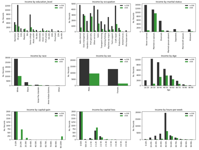
We first attempt to gain insight about the features that could be informative and discriminating and/or those that could provide the highest information gain, say using a "rule of thumb" or heuristic criterion. To this end we carry an exploratory analyss of each of the features and compute the underlying frequency distribution for each of the feature categories (subfeatures). See bar plots below (the generatinc code appears immmediately later following this section).
Analysis:
First, we can remove subsets of features from the training dataset and observe whether their removal maintains or improves our predictive performance metric. Features that don't affect performance metrics according to an established criterion or tolerance will be deemed irrelevant. Features that imply some form of redundancy or linear dependance on others would be removed accordingly as well.
Second, we can try to estimate the purity of the feature or sufeatures that split into the classes of interest. Let us take a look at the subplots given above, each representing a selected feature, e.g education, occupation, etc. For categorical features we identify subfeatures representing a unique value of the parent feature and which splits the data classes, '<=50K' (black color) and '>50K' (green color); for continuous data each subfeature represents an interval and each interval splits the data in the same corresponding classes.
Intuition from visual inspection ("rule of thumb"):
When targeting a specific feature, we aim to identify the subfeatures with the highest purity, i.e. a clear separation or discrimination between two classes of interest; preferentially in our case, observing a higher proportion of individuals earning '>50K' in some of the subfeatures, i.e taller green bars somewhere in the attribute distribution. A crude measure of this is the following ratio:
R =(No. '>50K')/(No. '<=50K') > threshold >= 0.5 (50%), or equivalently with largest group percentage: GP = (No. '>50K')/((No. '<=50K') + (No. '<=50K')).
In addition, the proportion of individuals belonging to a given class within a group should be representative of the total number of individuals earning '>50K'.
1. Age: The class distribution appears to be the envelope of a normal distribution, which is good for expectation values in relation to the '>50K' class. Near the center we have subfeatures corresponding to age groups 40-50, 50-60 with a significant proportion of '>50K', R >0.5.
2. Capital loss: This feature contains 3 subfeatures (capital gain amounts of 10-20K, 20-30K and 90-100K) with majority '>50K' class and clearly discriminated from the rest of the subfeatures. Among all features, capital gain fulfills all of our simplified feature importance criteria.
3. Capital gain: This feature contains 2 subfeatures (capital loss amounts of 1.5-2K, 2.5-3K) with majority '>50K' class and 1 subfeature (2-2.5K) with R > 50%. These attribute groups are clearly discriminated from the rest of the subfeatures. Capital loss fulfills all of our simplified feature importance criteria.
4. Hours per week: Contains the subfeatures "50-60h" and "60-70h" which contain a significant proportion of '>50K' earners, R >0.5. In addition, the "40-50h" groups seems discriminating, i.e. most people working 40 to 50 hours per week would earn less than 50K.
5. Education Level: It contains subfeatures "Masters", "Doctorate" and "Prof. School" with majority '>50K' class, and "Bachelors", with a high percentage of ">50K" earners in that group R > 0.5. Although these groups discriminate between the two income classes, the '>50K' (green) distribution spreads a bit more among the rest of the groups in comparison to capital gain and loss.
The rest of the features do not fulfill our "rule of thumb" criteria except for "Occupation" and "Civil Status", which contain several ">50K" groups with R>0.5, but no '>50K' majority groups. In addition, 'occupation' seems to be correlated or dependent on the education feature (possibly redundant).
#It generates bar plots indicating no. records per
#selected raw feature. Bars are split by the income threshold $50K
#Juan E. Rolon

import numpy as np
import pandas as pd
import matplotlib.pyplot as plt

sub_features = ['education_level', 'occupation', 'marital-status', 'race', 'sex']

#create figure
plt.figure(1, figsize=(16, 16))
plot_num = 1
nrows = 4
ncols = 3
for feat_choice in sub_features:
    groups = features_raw[feat_choice].unique()
    gelems = len(groups)
    less_than_50 = [0] * gelems
    more_than_50 = [0] * gelems
    for ocn in range(len(groups)):
        for row in range(len(features_raw)):
            if features_raw[feat_choice][row].strip() == groups[ocn].strip() and income_raw[row].strip() == '>50K':
                more_than_50[ocn] += 1
            elif features_raw[feat_choice][row].strip() == groups[ocn].strip() and income_raw[row].strip() == '<=50K':
                less_than_50[ocn] += 1

    # create subplots for 'education_level', 'occupation', 'marital-status', 'race', 'sex'
    plt.subplot(nrows, ncols, plot_num)
    index = np.arange(gelems)
    bar_width = 0.35
    opacity = 0.8
    rects1 = plt.bar(index, less_than_50, bar_width, alpha=opacity, color='k', label='<=50K')
    rects2 = plt.bar(index + bar_width, more_than_50, bar_width, alpha=opacity, color='g', label='>50K')
    plt.ylabel('No. Records')
    plt.title('Income by {}'.format(feat_choice))
    plt.xticks(index + bar_width / 2.0, groups, rotation='vertical')
    plt.legend(frameon=False, loc='upper right', fontsize='small')
    plot_num += 1

# create extra subplot for 'age'

age_groups = ['10-20', '20-30', '30-40', '40-50', '50-60', '60-70', '70-80', '80-90']
n_groups_age = len(age_groups)
less_than_50_age = [0] * n_groups_age
more_than_50_age = [0] * n_groups_age
d_age = 10
offset = 0
for agn in range(len(age_groups)):
    if agn == len(age_groups) - 1: offset = 1
    for row in range(len(features_raw)):
        if d_age <= features_raw['age'][row] < d_age + 10 + offset and income_raw[row].strip() == '>50K':
            more_than_50_age[agn] += 1
        elif d_age <= features_raw['age'][row] < d_age + 10 + offset and income_raw[row].strip() == '<=50K':
            less_than_50_age[agn] += 1
    d_age += 10

plt.subplot(nrows, ncols, plot_num)
index = np.arange(n_groups_age)
bar_width = 0.35
opacity = 0.8
rects1 = plt.bar(index, less_than_50_age, bar_width, alpha=opacity, color='k', label='<=50K')
rects2 = plt.bar(index + bar_width, more_than_50_age, bar_width, alpha=opacity, color='g', label='>50K')
plt.xlabel('Age')
plt.ylabel('No. Records')
plt.title('Income by Age')
plt.xticks(index + bar_width / 2.0, age_groups)
plt.legend(frameon=False, loc='upper right', fontsize='small')

# create extra subplot for 'capital-gain', 'capital-loss'

cap_gain_groups = ['0-10K', '10-20K', '20-30K', '30-40K', '40-50K', '50-60K', '60-70K', '70-80K', '80-90K', '90-100K']
cap_loss_groups = ['0-500', '500-1K', '1-1.5K', '1.5-2K', '2-2.5K', '2.5-3K', '3-3.5K', '3.5-4K','4-4.5K', '4.5-5K']
weekly_hours = ['0-10h', '10-20h', '20-30h', '30-40h', '40-50h', '50-60h', '60-70h', '70-80h','80-90h', '90-99h']
gr_set = [cap_gain_groups, cap_loss_groups, weekly_hours]
cap_feat = ['capital-gain', 'capital-loss', 'hours-per-week']

for m, feat in enumerate(cap_feat):
    n_groups_cap = len(gr_set[m])
    less_than_50 = [0] * n_groups_cap
    more_than_50 = [0] * n_groups_cap
    d_cap = 0
    steps = [10000, 500,10]
    offset = 0
    for agn in range(len(gr_set[m])):
        if agn == len(gr_set[m]) - 1: offset = 100
        for row in range(len(features_raw)):
            if d_cap <= features_raw[feat][row] < d_cap + steps[m] + offset and income_raw[row].strip() == '>50K':
                more_than_50[agn] += 1
            elif d_cap <= features_raw[feat][row] < d_cap + steps[m] + offset and income_raw[row].strip() == '<=50K':
                less_than_50[agn] += 1
        d_cap += steps[m]

    # create subplots
    plt.subplot(nrows, ncols, plot_num + 1)
    index = np.arange(n_groups_cap)
    bar_width = 0.35
    opacity = 0.8
    rects1 = plt.bar(index, less_than_50, bar_width, alpha=opacity, color='k', label='<=50K')
    rects2 = plt.bar(index + bar_width, more_than_50, bar_width, alpha=opacity, color='g', label='>50K')
    plt.title('Income by {}'.format(feat))
    plt.ylabel('No. Records')
    if feat in ['capital-gain', 'capital-loss']:
        plt.ylim((0, 2000))
    plt.xticks(index + bar_width / 2.0, gr_set[m], rotation='vertical')
    plt.legend(frameon=False, loc='upper right', fontsize='small')
    plot_num += 1

plt.tight_layout()
plt.show()

Extracting Feature Importances using Machine Learning
In this phase of our analysis we use machine learning techniques to determine which features provide the most predictive power. By focusing on the relationship between only a few crucial features and the target label we simplify our understanding of the underlying system mechanisms, which is most always a useful thing to do.
Again we wish to identify a small number of features that most strongly predict whether an individual makes at most or more than \$50,000.
To accomplish the feature selection process, we choose a scikit-learn classifierthat has a feature_importance_ attribute, which is a function that ranks the importance of features according to the chosen classifier.
In the next code cell, we fit this classifier to training set and use this attribute to determine the top 5 most important features for the census dataset.
Extracting Feature Importances.
We choose a scikit-learn supervised learning algorithm that has a feature_importance_ attribute availble for it. This attribute is a function that ranks the importance of each feature when making predictions based on the chosen algorithm.
In the code cell below, we implement the following:
- Import a supervised learning model from sklearn.
- Train the supervised model on the entire training set.
- Extract the feature importances using
'.feature_importances_'.
# TODO: Import a supervised learning model that has 'feature_importances_'
from sklearn.ensemble import GradientBoostingClassifier

# TODO: Train the supervised model on the training set using .fit(X_train, y_train)
model = GradientBoostingClassifier(n_estimators=200,random_state=10,max_depth=4)
model.fit(X_train,y_train)

# TODO: Extract the feature importances using .feature_importances_
importances = model.feature_importances_

# Plot
vs.feature_plot(importances, X_train, y_train)

Feature Importances Results
There is qualitative agreement between these results and those discussed in our exploratory analysis. In particular, the features "Age", "Capital-gain" and "Capital-loss" confirm our expectations regarding them as the features that have the largest weight and impact on the model's performance metrics.
The same comparison applies broadly to the "education" and "civil status" features. (Notice that sklearn refers to the "education number" assigned to the categorical attributes of the "education" feature; it is understood that they are equivalent).
We need to remark that sklearn feature selection is highly dependent on the hyperparameters passed to the classifier and/or the resulting optimized hyperparameters. In addition, sklearn feature weighing takes place over the full set of 103 scaled and encoded features, not over the original features being ranked.
In my opinion, feature selection over the final set of features makes more sense as several attributes whithin the main features (see bar plots) carry little information about the '>50K' class.
Feature Selection
In this phase of our analysis we want to find out how does a model perform if we only use a subset of all the available features in the data.
With less features required to train, the expectation is that training and prediction time is much lower — at the cost of performance metrics.
From the visualization above, we see that the top five most important features contribute more than half of the importance of all features present in the data. This hints that we can attempt to reduce the feature space and simplify the information required for the model to learn.
In the code cell below we use the same optimized model extracted earlier, and train it on the same training set with only the top five important features.
# Import functionality for cloning a model
from sklearn.base import clone

# Reduce the feature space
X_train_reduced = X_train[X_train.columns.values[(np.argsort(importances)[::-1])[:5]]]
X_test_reduced = X_test[X_test.columns.values[(np.argsort(importances)[::-1])[:5]]]

# Train on the "best" model found from grid search earlier
clf = (clone(best_clf)).fit(X_train_reduced, y_train)

# Make new predictions
reduced_predictions = clf.predict(X_test_reduced)

# Report scores from the final model using both versions of data
print "Final Model trained on full data\n------"
print "Accuracy on testing data: {:.4f}".format(accuracy_score(y_test, best_predictions))
print "F-score on testing data: {:.4f}".format(fbeta_score(y_test, best_predictions, beta = 0.5))
print "\nFinal Model trained on reduced data\n------"
print "Accuracy on testing data: {:.4f}".format(accuracy_score(y_test, reduced_predictions))
print "F-score on testing data: {:.4f}".format(fbeta_score(y_test, reduced_predictions, beta = 0.5))
#I generated this optional code cell to complement

#Juan E. Rolon
import matplotlib.pyplot as plt
clf = clone(best_clf)
clf_scores = []
clf_train_times = []
clf_names = []
features_train = [X_train, X_train_reduced]
features_test = [X_test, X_test_reduced]
temp_scores = []
temp_times = []
for i in range(len(features_train)):
    clf_results = train_predict(clf, len(y_train), features_train[i], y_train, features_test[i], y_test)
    clf_scores.append(clf_results['f_test'])
    clf_train_times.append(clf_results['train_time'])
clf_names = ['Final Model & Full Data', 'Final Model & Reduced Data']
print clf_scores
print clf_train_times

n_groups = len(clf_scores)
index = np.arange(n_groups)
bar_width = 0.35
opacity = 0.4

impdata1 = clf_scores
impdata2 = clf_train_times

plt.subplot(2, 1, 1)

plt.ylabel('F-Score Test ')
plt.xticks(index, clf_names)
bar1 = plt.bar(index, impdata1, bar_width, alpha=opacity, color='k')
for rect in bar1:
    height = rect.get_height()
    plt.text(rect.get_x() + rect.get_width()/2.0, height, '%f' % height, ha='center', va='top',color='b')

plt.subplot(2, 1, 2)

plt.ylabel('Train Times ')
plt.xticks(index, clf_names)
bar2 = plt.bar(index, impdata2, bar_width, alpha=opacity, color='g')
for rect in bar2:
    height = rect.get_height()
    plt.text(rect.get_x() + rect.get_width()/2.0, height, '%f' % height, ha='center', va='top',color='b')

plt.tight_layout()
plt.show()

Effects of Feature Selection
As shown in the bar plots above, feature selection produces a reduction on the performance metrics accuracy and f-score. In particular, there is a 1.2% reduction in accuracy and a 3.2% reduction in the f-score.
If training computing time is a factor we recommend using the reduced data model as it is an order of magnitude faster. I belive this improvement in training time would be worthwhile for training a much lager data set at the expense of just 3.2% reduction in the f-score.