Machine Learning Approach to the Discovery of Disease Risk Factors on Individuals Assessed by the National Health and Nutrition Examination Surveys 2013-2014¶

Juan E. Rolon¶

e-mail: rolon.math@gmail.com

Original capstone project submitted to Udacity, Inc. as partial fulfillment to obtain the certification as a Machine Learning Engineer.

Project Overview¶

The prediction of chronic disease risk factors is one of the most important and challenging problems in healthcare analytics [1]. Accurate risk factor prediction helps developing strategies aimed at avoiding unnecessary interventions for patients and reducing costs for insurance companies and healthcare providers.

An important step towards risk factor prediction is the identification of individuals who would benefit from preventive treatment. Machine-learning algorithms are strongly suited for this task as they can improve identification accuracy by exploiting complex interactions between different risk factors and patient data features associated to disease [2].

In particular, supervised and unsupervised learning techniques can be applied to extract risk-associated features from readily available healthcare data, including demographic and wellness data, lifestyle behavior and health status markers.

Among the chronic diseases that are the focus of intense research in the domain of healthcare analytics are diabetes and cardiovascular disease (CVD). In the United States, estimates indicate the existence of 30.3 million people with diabetes (9.4% of the US population) including 23.1 million people who are diagnosed and 7.2 million people (23.8%) undiagnosed. The numbers for prediabetes indicate that 84.1 million adults (33.9% of the adult U.S. population) have prediabetes, including 23.1 million adults aged 65 years or older (the age group with highest rate).

Furthermore, about 610,000 people die of cardiovascular disease in the United States every year, that is 1 in every 4 deaths. In particular, heart disease is the leading cause of death for both men and women [3, 4].

Problem Statement¶

We train a gradient boosting classifier on publicly available data, to identify risk predictors for diabetes and cardiovascular disease for individuals residing in the United States. Our results suggest that researchers and clinicians could make use of machine learning analyses to obtain valuable health assessment of patients at a much reduced cost and time.

The data for our study were extracted from a population sample of individuals who participated in the National Health and Nutrition Examination Surveys (NHANES) 2013-2014.

The present problem is framed as a binary classification task, in which the positive class are individuals presenting the disease, while the negative class are individuals not presenting the disease. The model's solution consists of the following components

1. Compilation and pre-processing of clinical datasets containing personal health status data.
2. Accurate classification of a surveyed person as having risk or no risk for a target disease.
3. Identification of important features (risk factors) that serve as main predictors of disease.

Datasets and Inputs¶

• The NHANES datasets contain unique records on demographic, health status, eating behavior and blood biochemistry data of surveyed individuals.

• The NHANES datasets are open source and unrestricted and are available to the public for download at the CDC National Center for Health Statistics at https://www.cdc.gov/nchs/nhanes/index.htm.

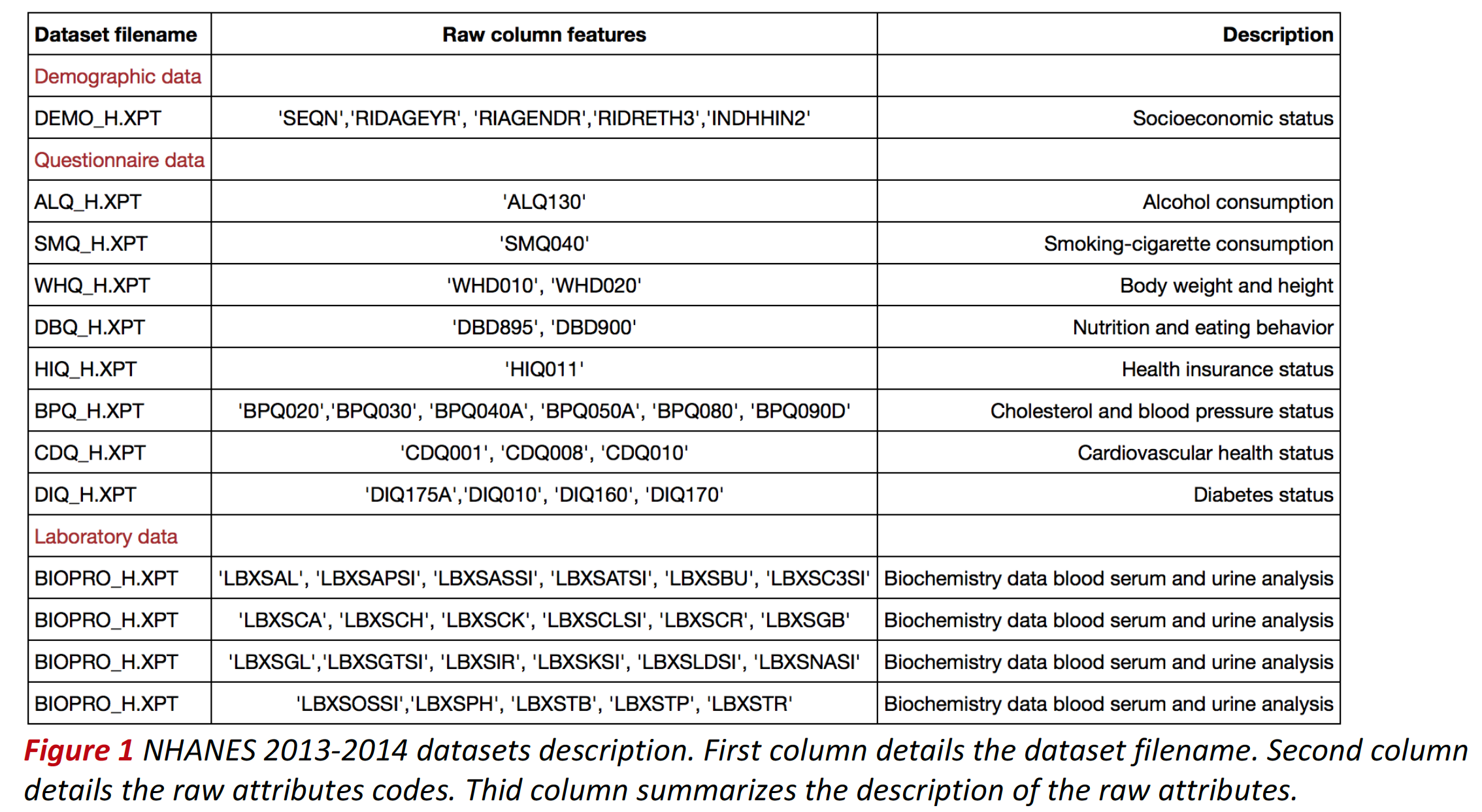
• Each NHANES 2013-2014 raw dataset is stored in SAS transport file format (XPT) and corresponds uniquely to a single questionnaire provided to respondents. Surveyed individuals are assigned a unique identifier number (SEQN) which serves as record index. The table below summarizes the datasets uses, the raw attributes and their description.

• Demographic and questionnaire column labels were renamed. The new labels were selected according to their description in the dataset documentation. Biochemistry feature column labels were not changed. See table below for the description of each label.

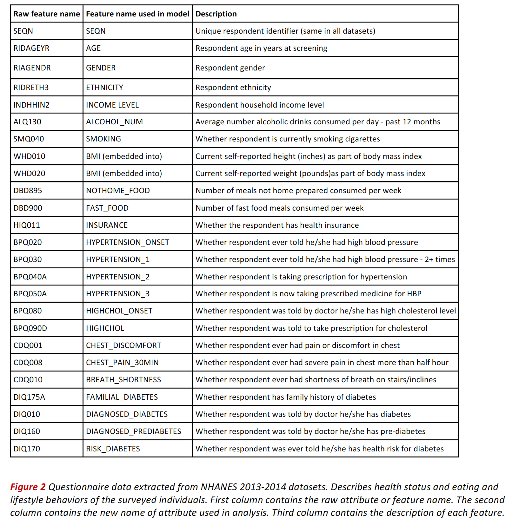
Health Status Questionnaire Data¶

The questionnaires gather health status and lifestyle behavior that we consider as potential predictors for cardiovascular disease and diabetes.

The table belows shows the colums and features corresponding to health status records.

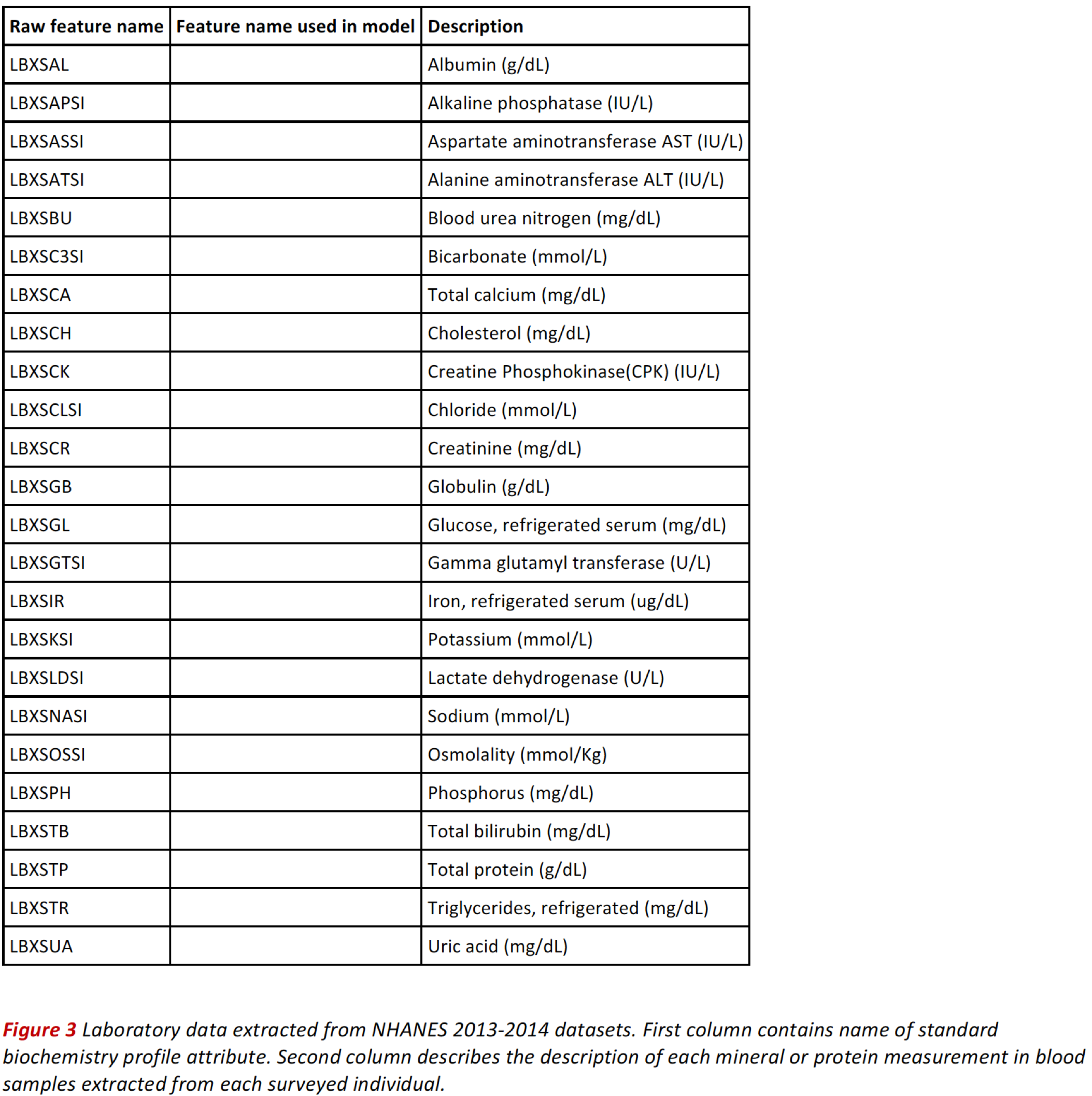
Blood Standard Biochemistry Data¶

Standard biochemistry data contains a series of measurements used in the diagnosis and treatment of certain liver, heart, and kidney diseases; acid-base imbalance in the respiratory and metabolic systems; other diseases involving lipid metabolism; various endocrine disorders; as well as other metabolic or nutritional disorders. We also consider these potential predictors for cardiovascular disease and diabetes.

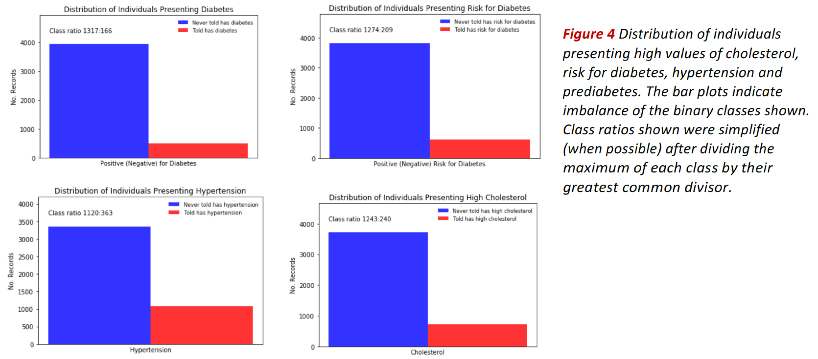
Data Exploration¶

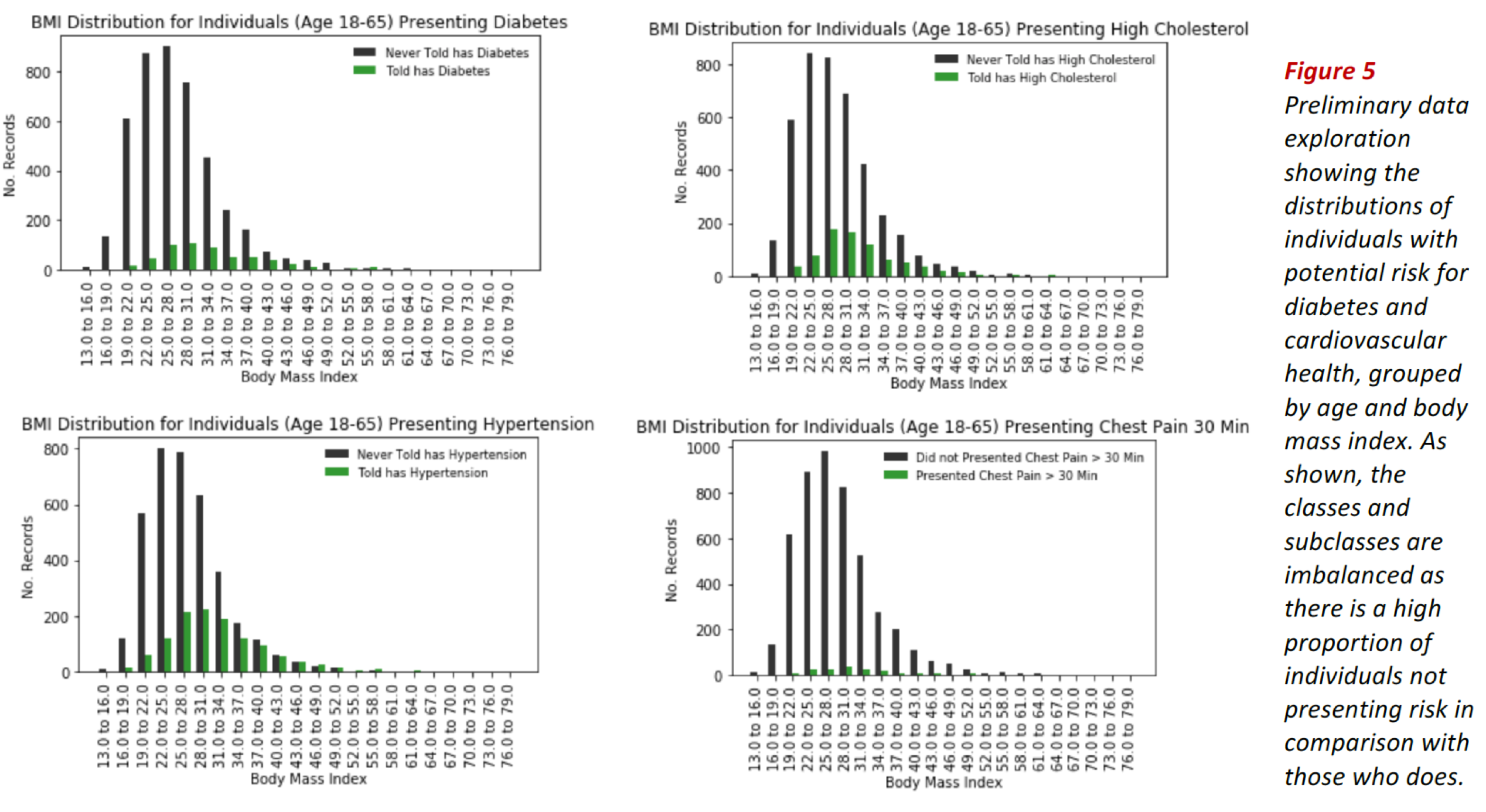
The bar plots in Fig. 4 show the distribution of individuals presenting high values of cholesterol, risk for diabetes, hypertension and prediabetes (see bars in red).

In all cases, the classes are imbalanced, as indicated by the corresponding class ratios. Class imbalance is also evidenced when we divide the data by groups, e.g. by age or body mass index as shown in Fig. 5.

These exploratory results suggest using classification evaluation metrics adequate for class imbalanced problems such as ROC-AUC score, recall, specificity, f1-score and illustrative tools such as confusion matrices and ROC curves.

Performance Metrics¶

We use AUC ROC as the primary metric to determine classification performance, while considering complementary metrics typically used in clinical settings. In our case, the target feature is a disease.

From the cohort of surveyed individuals is reasonable to assume that the prevalent class are the healthy subjects (negative cases), while the diseased belong to the rare class (positive cases). The rare class is the class of more interest, and is typically designated 1 (presenting disease), in contrast to the more prevalent 0s (not presenting disease).

Area Under ROC Curve.¶

• This is our main metric. ROC curve in itself doesn’t constitute a single measure for classifier performance. AUC is simply the total area under the ROC curve. The larger the value of AUC, the more effective the classifier.

• When using normalized units, AUC is equal to the probability that a classifier will rank a randomly chosen positive instance higher than a randomly chosen negative one (assuming 'positive' ranks higher than 'negative').

ROC Curve¶

• A plot of recall vs. specificity. For problems with imbalanced classes there is always trade-off between recall and specificity as we change the cutoff to determine how to classify a record. This indicator is directly related to the ROC-AUC score.

Confusion Matrix¶

As shown in Fig. 6, the confusion matrix is a table showing the number of correct and incorrect predictions categorized by type of response. This indicator is directly related to the metrics precision, recall, specificity and f1-score.

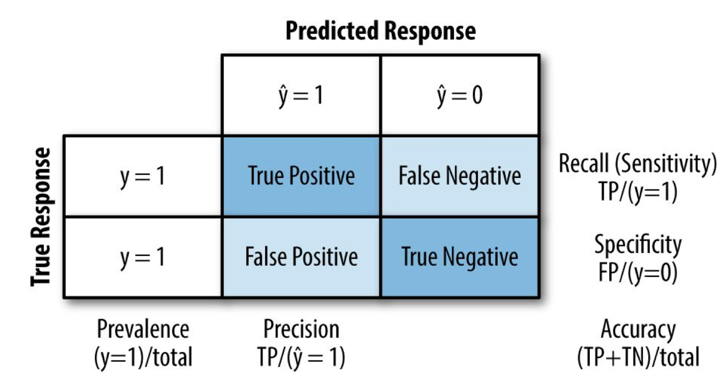
Figure 6 Confusion matrix schematics showing some of the related metrics considered in this work.

Recall¶

• This metric measures the strength of the model to predict a positive outcome (disease) — the proportion of the 1s that it correctly identifies.

$$ \it Recall = \frac{\sum \text{True Positives}}{\sum \text{True Positives} + \sum \text{False Negatives} } $$

Specificity¶

• This metric measures the strength of the model to predict a negative outcome (no presenting disease) — the proportion of the 0s that it correctly identifies.

$$ \it Recall = \frac{\sum \text{True Negatives}}{\sum \text{True Negatives} + \sum \text{False Negatives} } $$

Precision¶

• This metric measures the accuracy of a predicted positive outcome (presenting disease).

$$ \it Recall = \frac{\sum \text{True Positives}}{\sum \text{True Positives} + \sum \text{False Positives} } $$

Accuracy¶

• This metric measures the accuracy of a predicted positive outcome (presenting disease).

$$ \it Recall = \frac{\sum \text{True Positives} +\sum \text{True Negatives}}{\sum \text{True Positives} + \sum \text{False Positive} +\sum \text{True Negatives} + \sum \text{False Negatives} } $$

$F_1$ score¶

• This metric is the harmonic average of the precision and recall, reaching its best value at 1 (perfect precision and recall) and worst at 0.

$$ 2 \times \frac{\text{Precision}\times\text{Recall}}{\text{Precision}+\text{Recall}} $$

Algorithms and Techniques¶

Classification Algorithm¶

To solve our classification problem, we make use of XGBoost (Extreme Gradient Boosting), which is an optimized distributed gradient boosting library designed to be highly efficient, flexible and portable. It implements machine learning algorithms under the Gradient Boosting framework [7].

More generally, Gradient Boosting is an ensemble machine learning technique for regression and classification problems, which produces a prediction model in the form of an ensemble of weak prediction models (typically decision trees for XGBoost). Gradient boosting is an approach where new models are created that predict the residuals or errors of prior models and then added together to make the final prediction. It is called gradient boosting because it uses a gradient descent algorithm to minimize the loss when adding new models [8].

Main justifications for the problem at hand:

1. Faster than normal Gradient Boosting as it implements parallel processing.
2. Useful for unbalanced classes. Controls the balance of the positive and negative weights, via scale_pos_weight hyper-parameter tuning.
3. Ability to use AUC for optimization and evaluation.
4. Provides a built-in feature importance ranking algorithm.
5. Scalable to big-data applications. Permits scaling up the problem discussed in this project for the case of integrating larger healthcare datasets from multiple sources.

Feature Extraction¶

To identify the important features i.e. risk factors that serve as main predictors of disease, we use a feature importance measure built-in within the XGBoost framework. This measure is calculated for a single decision tree using the F-score, which is the amount that each attribute split point improves the performance measure (AUC), weighted by the number of observations the node is responsible for.

Generally, the feature importance score indicates how useful or valuable each feature was in the construction of the boosted decision trees within the model. The more an attribute is used to make key decisions with decision trees, the higher its relative importance.

Optimization techniques¶

Incremental Grid Search with Cross Validation¶

We implemented optimization of Xgboost hyper-parameters using cross-validated grid search, methodically building and evaluating a model for each combination of parameters specified in a grid. To control for overfitting, a stratified k-fold cross validation was applied in each iteration of grid-search.

Synthetic Minority Oversampling Technique (SMOTE)¶

We tested this technique to create synthetic data with aim of mitigating class imbalance. SMOTE selects two or more similar data instances (using a distance measure) and perturbing an instance one attribute at a time by a random amount within the difference to the neighboring instances. SMOTE can achieve better classifier performance (in ROC space).

Auxiliary testing algorithms¶

Preprocessing and scaling. We developed and implemented a series of algorithms to perform all the necessary data cleaning, feature scaling and visualization.

Datasets Preprocessing¶

The data preprocessing step was the most time-consuming in the present project. Given the imbalanced nature of the classification problem at hand, it is critical that the curated dataset contains enough and consistent record values expressed in a useful scale and format. Also, we want to consider only the features relevant to our problem. The following preprocessing pipeline was implemented:

General procedure¶

• Read each SAS file and convert it to a pandas dataframe.

• Restrict dataframe to relevant features.

• Identify codes representing missing value (different SAS datasets use different codes for missing values).

• Data imputation. Remove missing values or replace missing values with zeroes, or mean values when appropriate.

• Mitigate dataset biasing by imputation procedures. Data imputation on missing values was done after ensuring they were less than 10% of data; in any other case, data was done with mean values when appropriate. In some instances, we removed entire rows when several missing values occurred across columns.

• One hot encoding of categorical features when appropriate.

• Recoding and reordering ordinal features when not ordered in original dataset.

• Perform normalization and feature scaling according to the nature of the data presented in each data set. This step necessitated the creation of custom processing algorithms to achieve scaling appropriate for each dataset.

• Ensure dataframes consistency in terms equal number of records.

• Integrate all dataframes into a single consistent dataframe free of missing values, with all features appropriately re-scaled.

Modeling Workflow¶

The figure below shows our implementation flow chart indicating the processes and algorithms involved in determining the most important features that predict the risk for cardiovascular disease and diabetes.

Figure 7 Modeling workflow leading to the results discussed in the present report.

Preliminary Analysis¶

Correlation Matrices and Heatmaps¶

To gain preliminary insight about important predictors for CVD and Diabetes, we constructed a pair of correlation matrices. The correlations were computed using point biserial correlation coefficient. The point biserial correlation coefficient pointbiserialr(Y,X) is a correlation coefficient used when one variable Y is dichotomous (binary) and the other X is either continuous or dichotomous [9].

The figure below shows a correlation heat map indicating the correlation between health status features as defined in questionnaire data records.

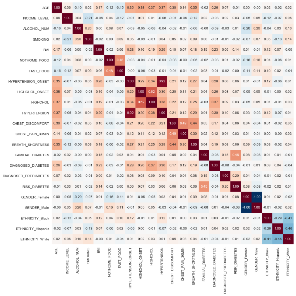Figure 8 Correlation matrix heat map showing the correlation among health-status conditions. Positive correlation is highlighted in orange tones; negative correlation is highlighted with blue tones. Each matrix element is a point biserial correlation measure. In particular, we notice a cluster of high positive correlation between Hypertension onset, High Cholesterol Onset, High Cholesterol, Hypertension, Chest discomfort, Chest Pain and Shortness of Breath, which collectively conform the signatures of Cardiovascular Disease (CVD); the weighted sum of this features corresponds to the CVD target label 'CARDIO_DISORDER' as defined in the text.

The following observations highlight the validity of preliminary results, and indicate robust data quality:

• In particular, we notice a cluster of high positive correlation (center of heat map) between Hypertension Onset, High Cholesterol Onset, High Cholesterol, Hypertension, Chest discomfort, Chest Pain and Shortness of Breath, which collectively conform the signatures of Cardiovascular Disease (CVD).

• Using this insight, we engineered the CVD target label 'CARDIO_DISORDER' defined as the text the weighted sum of 'BREATH_SHORTNESS', 'CHEST_PAIN_30MIN', 'CHEST_DISCOMFORT', 'HYPERTENSION', and 'HYPERTENSION_ONSET'.

• 'AGE', 'BMI', DIAGNOSED_DIABETES' shows a significant positive correlation with these components. Indicating relationship between CVD and increased age and increased body mass index (obesity). Coupled to the above, 'FAST_FOOD', and 'NOT_HOME_FOOD' (a person's habit to eat pre-processed foods) correlates negatively with CVD indicators.

The figure below shows a correlation heat map showing the correlation between standard biochemistry profile features and features related to CVD and Diabetes predictors.

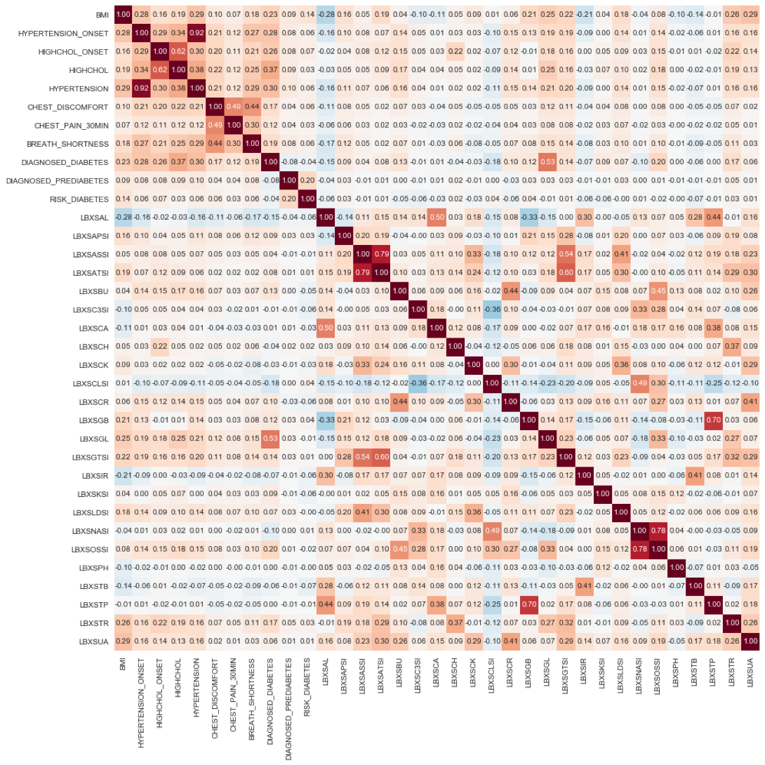Figure 9 Correlation matrix heat map showing the correlation between blood biochemistry features and features related to CVD and Diabetes predictors. Positive correlation is highlighted in orange tones; negative correlation is highlighted with blue tones.

The following observations highlight the validity of the preliminary results, and indicate excellent robust data quality:

• Again, we notice the same cluster of high positive correlation among CVD and Diabetes predictors shown in Fig. 12, but now located on the left upper corner of the heat map.

• 'LBXSGL' (Glucose level) positively correlates strongly with 'DIAGNOSED_DIABETES'

• 'LBXSAL' (Albumin level) negatively correlates with the CVD and Diabetes predictors, BMI, High Cholesterol Onset, High Cholesterol, Hypertension, Chest discomfort, Chest Pain and Shortness of Breath. Low albumin blood levels, even low normal, correlate with cellular inflammation and increased risk of death from cardiovascular disease (CVD,) such as coronary heart disease and strokes [https://labtestsonline.org/tests/albumin].

• 'LBXSCLSI' negatively correlates with the CVD and Diabetes predictors. A decreased level of blood chloride (called hypochloremia) occurs with any disorder that causes low blood sodium. Hypochloremia also occurs with congestive heart failure.

Classifier Implementation and Optimization¶

The XGBOOST classifier algorithm is trained on the health status and blood biochemistry data to classify a person as presenting or not the (risk of) disease, e.g. Cardiovascular Disease ('CARDIO_DISORDER') or Diabetes ('DIAGNOSED_DIABETES').

For each target label e.g. 'CARDIO_DISORDER', 'DIAGNOSED_DIABETES', we implemented a separate model and for each model we developed Grid-search Cross-Validation pipeline, for hyper-parameter tuning, i.e. each classification problem has their own set of optimal parameters, aimed at yielding the highest ROC-AUC score, while maintaining reasonable values of accuracy, specificity, precision and recall.

The function signature of the implemented XGBOOST classifier reads as follows:

model = xgb.XGBClassifier(learning_rate, n_estimators, max_depth, reg_alpha, min_child_weight, gamma, subsample, colsample_bytree, scale_pos_weight, objective)

The learning task is set by the objective parameter, which specifies the learning task and the corresponding learning objective or a custom objective function to be used. We use the objective binary:logistic (logistic regression for binary classification). It returns predicted probability of belonging to either of the two classes (1) or (0). To obtain the class, we round up the probability.

The following hyper-parameters were optimized using sklearn's GridSearchCV:

learning_rate. Boosting learning rate. Makes the model more robust by shrinking the weights on each step. Typical final values of this parameter are: 0.01-0.2.

n_estimators. Number of boosted trees to fit. Number depends on the complexity, scale and dimensionality of the problem.

max_depth. Maximum tree depth for base learners. Used to control overfitting as higher depth will allow model to learn relations very specific to a particular sample. Should be tuned using GridSearchCV. Typical values are: 3-10.

reg_alpha. L1 regularization term on weights. Tuned to compensate curse of dimensionality effects so that the algorithm runs faster when implemented.

min_child_weight. Minimum sum of instance weight needed in a child node. Used to control over-fitting. Higher values prevent a model from learning relations which might be highly specific to the particular sample selected for a tree. Extreme high values can lead to under-fitting hence. Recommended to be tuned using GridSearchCV.

gamma. Minimum loss reduction required to make a further partition on a leaf node of the tree. A node is split only when the resulting split gives a positive reduction in the loss function. Gamma specifies the minimum loss reduction required to make a split. Makes the algorithm conservative. The values can vary depending on the loss function and should be tuned.

subsample. Subsample ratio of the training instance. Denotes the fraction of observations to be randomly samples for each tree. Lower values make the algorithm more conservative and prevents overfitting but too small values might lead to under-fitting. Typical values are: 0.5-1.

colsample_bytree. Subsample ratio of columns randomly sampled when constructing each tree. Typical values: 0.5-1.

scale_pos_weight. Controls the balance of positive and negative weights, useful for unbalanced classes. A typical value to consider: sum(negative cases) / sum(positive cases).

The table below shows the results of the GridSearch optimization:

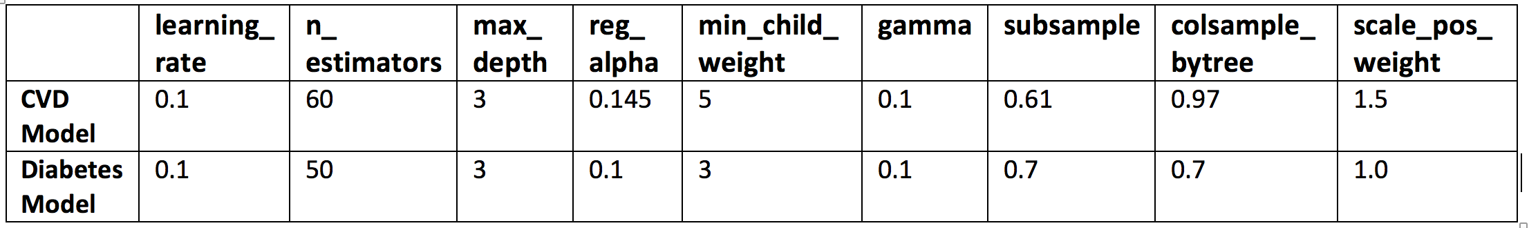Table 1 GridSearchCV optimization results.

Implemented Models¶

For each target disease with tested five XGBoost classifiers:

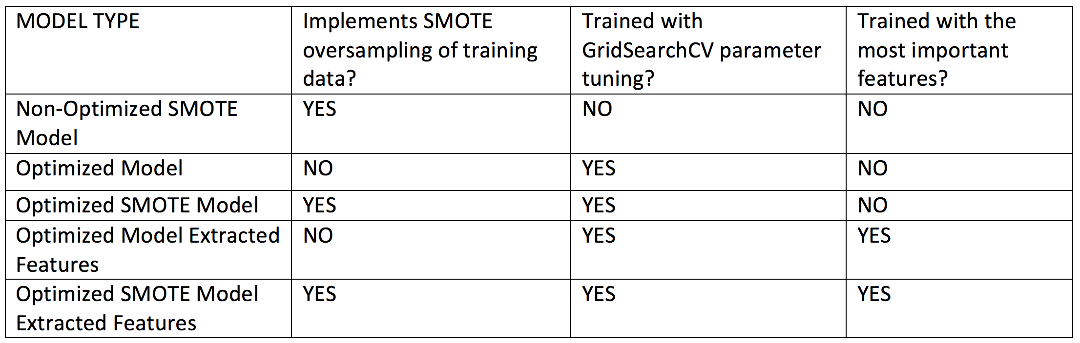Table 2 Implemented models. For models indicating use of extracted features, we retrained the optimized algorithms using a sub-selection of the most important features obtained using the f-score ranking scheme built-in in XGBoost, as shown in the bar plots in the Results section.

Results¶

Cardiovascular Disease (CVD) Risk Predictor Features¶

Below we summarize the dataset features used to train the XGBoost classifier to classify individuals as presenting or not (or dveloping risk) CVD.

Number of cases: 1469

Target label: CARDIO_DISORDER

Total input features for training: 32

Blood biochemistry features: 17

LBXSAL, LBXSAPSI, LBXSATSI, LBXSBU, LBXSCH, LBXSCK, LBXSCLSI, LBXSCR, LBXSGB, LBXSGL, LBXSGTSI, LBXSIR, LBXSKSI, LBXSLDSI, LBXSPH, LBXSTR, LBXSUA

Health status features: 15

AGE, INCOME_LEVEL, SMOKING, BMI, NOTHOME_FOOD, FAST_FOOD, HIGHCHOL_ONSET, HIGHCHOL, FAMILIAL_DIABETES, DIAGNOSED_DIABETES, RISK_DIABETES, GENDER_Female, GENDER_Male, ETHNICITY_Black, ETHNICITY_Hispanic, ETHNICITY_White

Classifier Performance Metrics¶

The table below summarizes the performance metrics assessed for each of the model implementations considered for CVD.

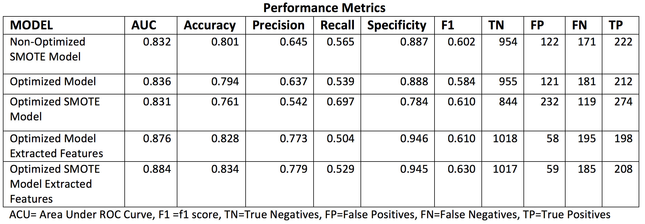Table 3 . Classifier performance metrics assess for the different implemented CVD models.

Receiver Operating Characteristic Curves¶

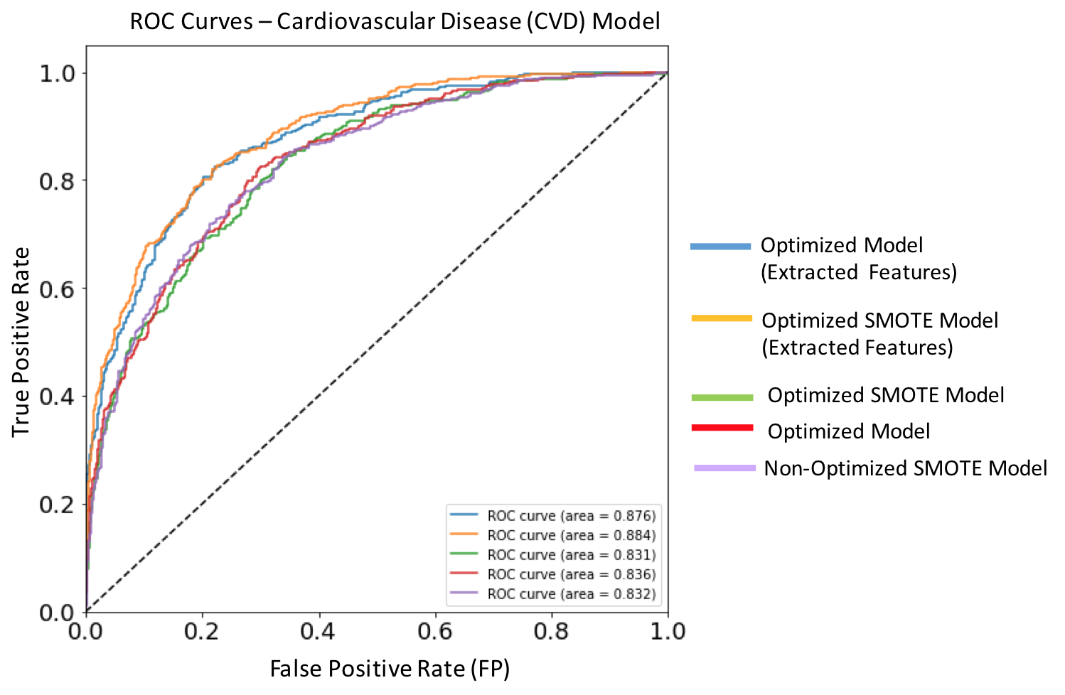Figure 10. ROC curves for each of the implemented XGBoost models targeting cardiovascular disease. Dashed diagonal line corresponds to a non-diagnostic random classifier. The model with best performance metric (orange solid line) is the optimized SMOTE model trained on extracted features, and has an AUC score of 0.884.

Feature Importances¶

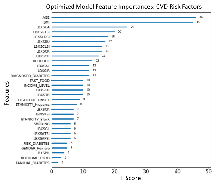Figure 11. F-score ranked feature importances obtained with optimized model trained on SMOTE oversampled data. The features with the largest scores represent the main important predictors for cardiovascular disease (CVD). In this model, Glucose (LBXSGL), Body mass index (BMI), Age (AGE), Creatinine (LBXSCR), Presenting a cardiovascular disorder (CARDIO_DISORDER), Diagnosed high cholesterol (HIGHCHOL), Cholesterol (LBXSCH), Albumin (LBXSAL), Familial diabetes history (FAMILIAL_DIABETES) and Potassium level (LBXSKSI), are the main ten risk predictors of diabetes.

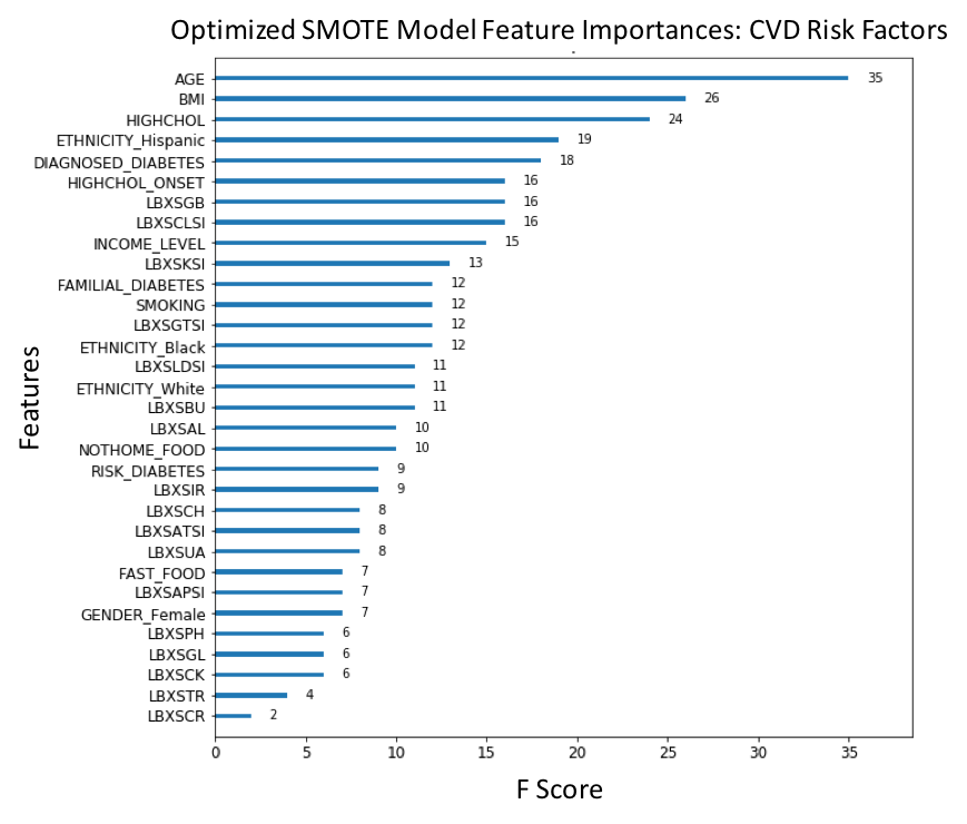Figure 12. F-score ranked feature importances obtained with optimized model for CVD trained on selected features. The features with the largest scores represent the main important predictors for cardiovascular disease (CVD). In this model, Body mass index (BMI), Age (AGE), Uric acid levels (LBXSUA), Creatinine (LBXSCR), Chloride (LBXSCLSI), Cholesterol (LBXSCH), Lactate dehydrogenase (LBXSLDSI), Gamma glutamyl transferase (LBXSGTSI), Blood urea nitrogen (LBXSBU) and Diagnosed high cholesterol (HIGHCHOL), are the main ten risk predictors of CVD. . (For each unique F-score, we can assign an ordinal rank N=1,2,3,.., where N=1 corresponds to the feature of largest importance score; this scheme is used to compare feature ranking in benchmark models).

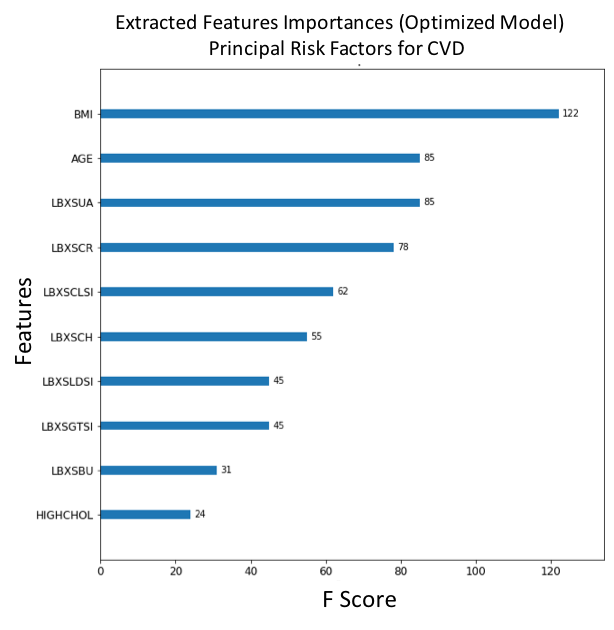Figure 13. F-score ranked feature importances obtained with optimized model trained on SMOTE oversampled data. The features with the largest scores represent the main important predictors for cardiovascular disease (CVD). In this model, Age (AGE), Body mass index (BMI), Diagnosed high cholesterol (HIGHCHOL), Being Hispanic (ETHNICITY_Hispanic), Diagnosed diabetes (DIAGNOSED_DIABETES), Diagnosed onset of high cholesterol (HIGHCHOL_ONSET), Globulin (LBXSGB), Chloride (LBXSCLSI), Income level (INCOME_LEVEL) and Potassium (LBXSKSI) are the main ten risk predictors of CVD. . (For each unique F-score, we can assign an ordinal rank N=1,2,3,.., where N=1 corresponds to the feature of largest importance score; this scheme is used to compare feature ranking in benchmark models).

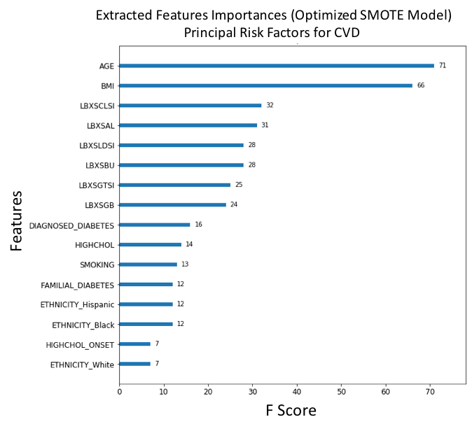Figure 14. F-score ranked feature importances obtained with optimized model trained on SMOTE oversampled selected features. The features with the largest scores represent the main important predictors for cardiovascular disease (CVD). In this model, Age (AGE), Body mass index (BMI), Chloride (LBXSCLSI), Albumin (LBXSAL), Lactate dehydrogenase (LBXSLDSI), Blood urea nitrogen (LBXSBU), Gamma glutamyl transferase (LBXSGTSI), Globulin (LBXSGB), Diagnosed diabetes (DIAGNOSED_DIABETES) and Diagnosed high cholesterol (HIGHCHOL), are the main ten risk predictors of CVD. (For each unique F-score, we can assign an ordinal rank N=1,2,3,.., where N=1 corresponds to the feature of largest importance score; this scheme is used to compare feature ranking in benchmark models).

Diabetes Risk Predictor Features¶

Below we summarize the dataset features used to train the XGBoost classifier to classify individuals as presenting or not (or dveloping risk) diabetes.

Number of cases: 1469

Target label: DIAGNOSED_DIABETES

Total input features for training: 24

Blood biochemistry features: 10

LBXSAL, LBXSATSI, LBXSBU, LBXSCLSI, LBXSCR, LBXSGL, LBXSGTSI, LBXSKSI, LBSOSSI, LBXSTR

Health status features: 14

AGE, ALCOHOL_NUM, SMOKING, BMI, FAST_FOOD, HYPERTENSION_ONSET, HIGHCHOL_ONSET, HIGHCHOL, HYPERTENSION, FAMILIAL_DIABETES, GENDER_Female, GENDER_Male, ETHNICITY_Black, ETHNICITY_Hispanic, ETHNICITY_White

Classifier Performance Metrics¶

The table below summarizes the performance metrics assessed for each of the model implementations considered for diabetes.

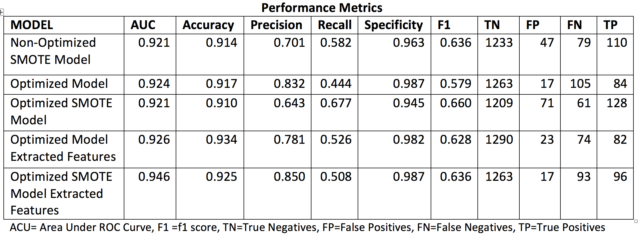Table 4. Classifier performance metrics assess for the different implemented Diabetes models.

Receiver Operating Characteristic Curves¶

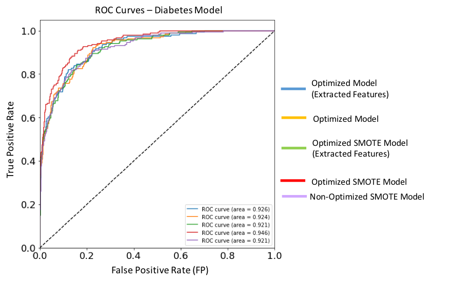Figure 15. ROC curves for each of the implemented XGBoost models targeting Diabetes. Dashed diagonal line corresponds to a non-diagnostic random classifier. The model with best performance metric (red solid line) is the optimized SMOTE model, and has an AUC score of 0.946.

Feature Importances¶

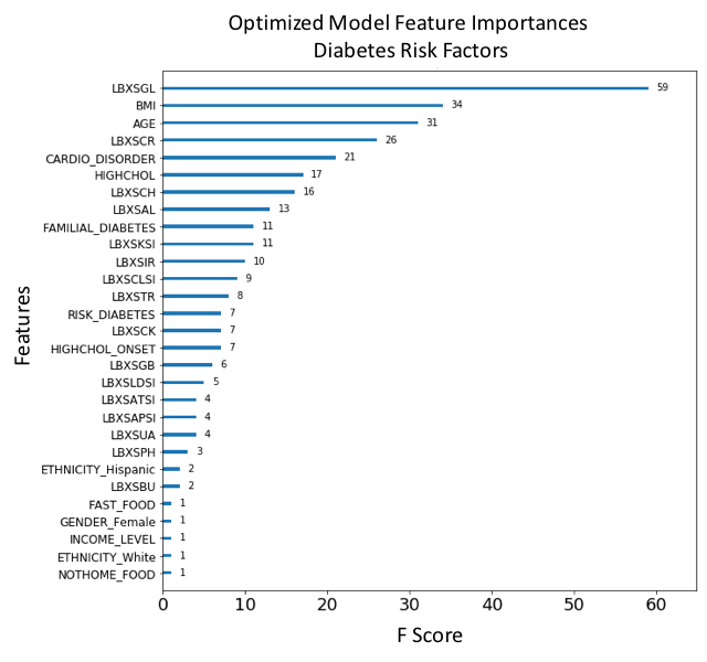Figure 16. F-score ranked feature importances obtained with optimized model trained on SMOTE oversampled data. The features with the largest scores represent the main important predictors for cardiovascular disease (CVD). In this model, Glucose (LBXSGL), Body mass index (BMI), Age (AGE), Creatinine (LBXSCR), Presenting a cardiovascular disorder (CARDIO_DISORDER), Diagnosed high cholesterol (HIGHCHOL), Cholesterol (LBXSCH), Albumin (LBXSAL), Familial diabetes history (FAMILIAL_DIABETES) and Potassium level (LBXSKSI), are the main ten risk predictors of diabetes.

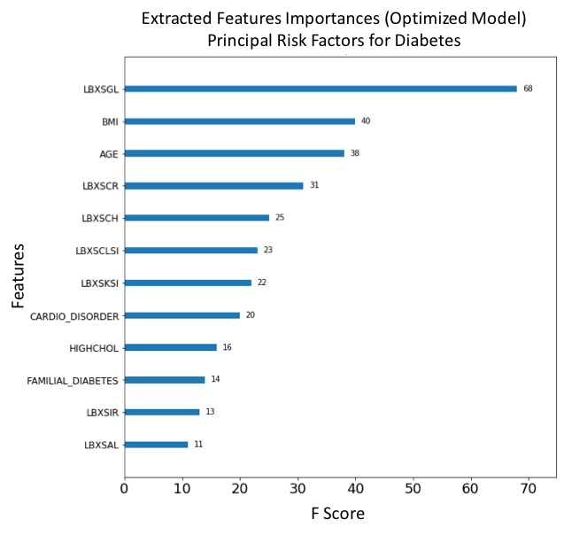Figure 17. F-score ranked feature importances obtained with optimized model trained on SMOTE oversampled selected features. The features with the largest scores represent the main important predictors for cardiovascular disease (CVD). In this model, Glucose (LBXSGL), Body mass index (BMI), Age (AGE), Creatinine (LBXSCR), Cholesterol (LBXSCH), Chloride (LBXSCLSI), Potassium (LBXSKSI), Presenting a cardiovascular disorder (CARDIO_DISORDER), Diagnosed high cholesterol (HIGHCHOL), Familial diabetes history (FAMILIAL_DIABETES), Iron (LBXSIR) and Albumin (LBXSAL) are the main risk predictors of diabetes.

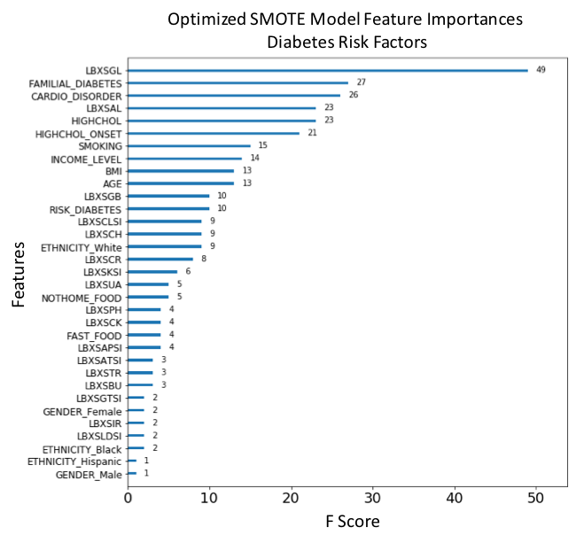Figure 18. F-score ranked feature importances obtained with optimized model trained on SMOTE oversampled data. The features with the largest scores represent the main important predictors for diabetes. In this model, Glucose (LBXSGL), Familial diabetes history (FAMILIAL_DIABETES), Presenting a cardiovascular disorder (CARDIO_DISORDER), Albumin (LBXSAL), Diagnosed high cholesterol (HIGHCHOL), High cholesterol onset (HIGHCHOL_ONSET), Smoking (SMOKING), Income level (INCOME_LEVEL), Body mass index (BMI) and Age (AGE), are the main risk predictors of diabetes.

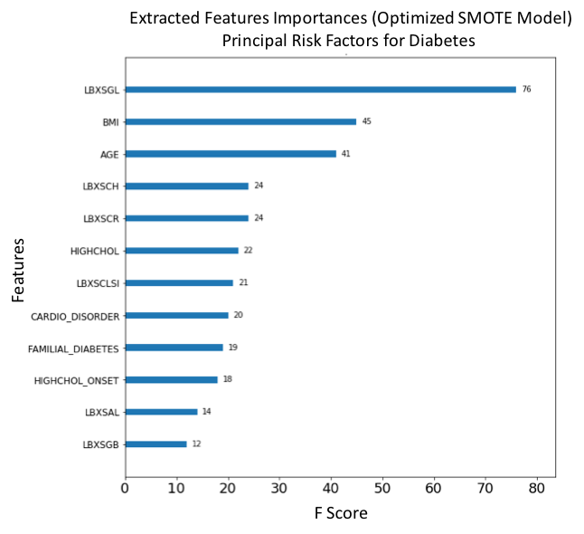Figure 19. F-score ranked feature importances obtained with optimized model trained on SMOTE oversampled selected features. The features with the largest scores represent the main important predictors for diabetes. In this model, Glucose (LBXSGL), Body mass index (BMI), Age (AGE), Cholesterol (LBXSCH), Creatinine (LBXSCR), Diagnosed high cholesterol (HIGHCHOL), Chloride (LBXSCLSI), Presenting a cardiovascular disorder (CARDIO_DISORDER), Familial diabetes history (FAMILIAL_DIABETES), High cholesterol onset (HIGHCHOL_ONSET), Albumin (LBXSAL) and Globulin level (LBXSGB) are the main risk predictors of diabetes.

Analysis and Justification¶

The main points that justify our results is their qualitative agreement with benchmark results and consistency with well-established clinical criteria regarding cardiovascular disease and diabetes risk factors. We will focus on the consistency of feature importance ranking across models.

As shown in Table 5, the disease risk predictors obtained by feature selection in our model strongly match those obtained in the benchmark models. For CVD, the features Age, BMI, Smoking, Ethnicity, Cholesterol, Glucose and Triglycerides are the most consistent risk predictors across models.

For diabetes, the features Age, Cardiovascular disorders, BMI (degree of obesity) and Smoking are the most consistent; (we notice the absence of an equivalent to Glucose (LBXSGL) in the benchmark model, this feature was not studied by M. Alghamdi, et al.).

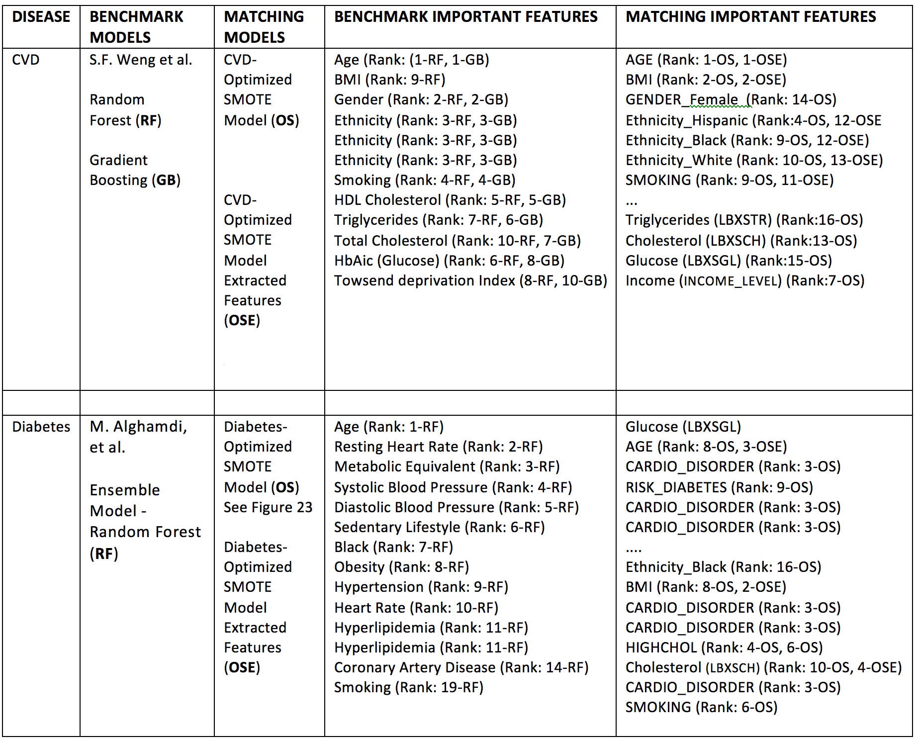Table 5. Qualitative comparison of feature importance rankings between refined models and benchmark models. Model codes refer to compared models (GB, RF, OS, OSE), see description in table. The feature ranks are expressed here using ordinal numbers N=1,2,3,.., e.g. Rank: N-MODEL CODE, where N=1 corresponds to the feature of largest importance score according to the particular score used, i.e. F-score, Gini coefficient, etc.

Table 6 below shows the performance comparison of selected XGBoost classifier models and benchmarks. We compare only the available metrics across models.

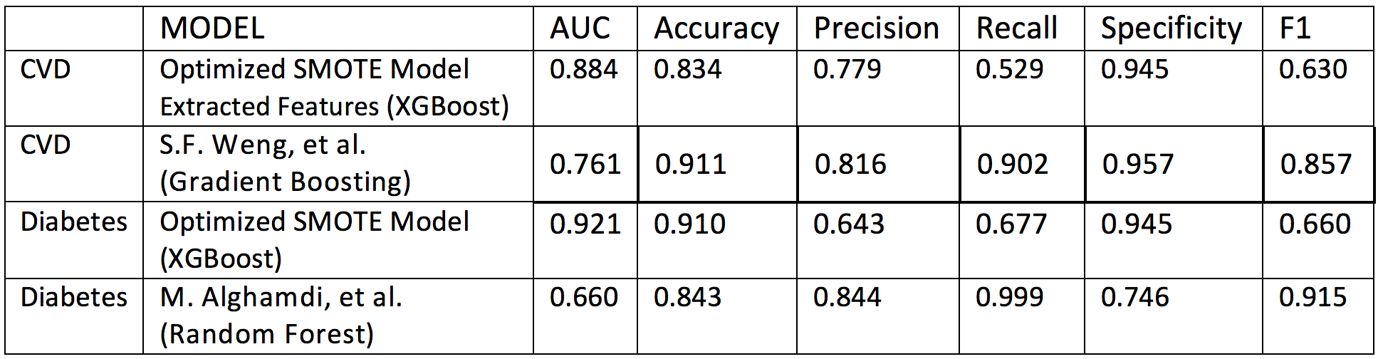Table 6. Performance comparison betwee selected XGBoost classifier models and benchmark models.

The following points are noted:

• For both, CVD and diabetes, ROC AUC scores in our models are superior to the benchmarks. This came at the expense of decreasing recall and f1 scores, which are greater (possibly optimized) in the benchmark models.

• Accuracy and precision scores are comparable across all models, except in our diabetes model, for which we obtained moderate gains in recall and f1 scores at the expense of decreased precision.

• Specificity is comparable across models, except for the benchmark diabetes model which underperforms in this measure at the expense of almost perfect recall and excellent f1 score; we also notice a poor AUC performance of this benchmark model.

Conclusions¶

We have shown how to utilize a AUC-optimized gradient boosting classifier to obtain important risk predictors for disease using feature importance measures.

Although, by using a much smaller dataset in comparison to scaled-up models, we have obtained results which are in strong qualitative and semi-quantitative agreement with the benchmarks.

Our results are also consistent with the clinical literature. This further strengthens the notion that machine learning models can be applied to aid in medical diagnosis by mining healthcare data to discover disease risk predictors.

The results of this project can be potentially improved by the following:

• Assembling a larger dataset by integrating the remaining NHANES surveys available at the US CDC. This will greatly reflect in all performance measures, in particular decreasing the number of false negatives in our model.

• Scaling-up the feature space by integrating other relevant features present in related datasets.

• Probing alternative oversampling strategies and different classifier models capable increasing the signal to noise ratio, e.g. deep neural-network based classifiers.

• Implementing longer and heterogeneous training pipelines combining the power of several different classifiers.

Bibliography¶

[1] K. Deepika and S. Shedole, Predictive analytics to prevent and control chronic diseases, 2016 2nd International Conference on Applied and Theoretical Computing and Communication Technology (iCATccT), 381-386. 10.1109/ICATCCT.7912028 (2016). Open Access Preprint

[2] M. Chen, Y. Hao, K. Hwang, L. Wang, Disease prediction by machine learning over big data from healthcare communities, IEEE Access, 5 (1), 8869-8879 (2017). https://doi.org/10.1109/ACCESS.2017.2694446

[3] The International Diabetes Federation. https://www.idf.org.

[4] US CDC Division for Heart Disease and Stroke Prevention. https://www.cdc.gov/dhdsp/data statistics/index.htm.

[5] S.F. Weng, J. Reps, J. Kai, J.M. Garibaldi, N. Qureshi, Can machine-learning improve cardiovascular risk prediction using routine clinical data?. PLOS ONE 12(4) e0174944 (2017). https://doi.org/10.1371/journal.pone.0174944.

[6] M. Alghamdi, M. Al-Mallah, S. Keteyian, C. Brawner, J. Ehrman, et al., Predicting diabetes mellitus using SMOTE and ensemble machine learning approach: The Henry Ford Exercise Testing (FIT) project, PLOS ONE 12(7) e0179805 (2017). https://doi.org/10.1371/journal.pone.0179805.

[7] Xgboost (https://en.wikipedia.org/wiki/Xgboost); A Gentle Introduction to XGBoost for Applied Machine Learning (https://machinelearningmastery.com/gentle-introduction-xgboost-applied-machine-learning).

[8] Gradient Boosting (https://en.wikipedia.org/wiki/Gradient_boosting); A Gentle Introduction to the Gradient Boosting Algorithm for Machine Learning (https://machinelearningmastery.com/gentle-introduction-gradient-boosting-algorithm-machine-learning).

[9] Point-biserial correlation coefficient (https://en.wikipedia.org/wiki/Point-biserial_correlation_coefficient).

---

Appendix 1: Benchmark Models¶

Our learning algorithms are benchmarked qualitatively and semi-quantitatively with recent algorithms developed by Weng [5] and Alghamdi [6]. These authors conducted analyses on big clinical datasets and ranked the most important risk factors for developing diabetes and cardiovascular disease using a large cohort of individuals.

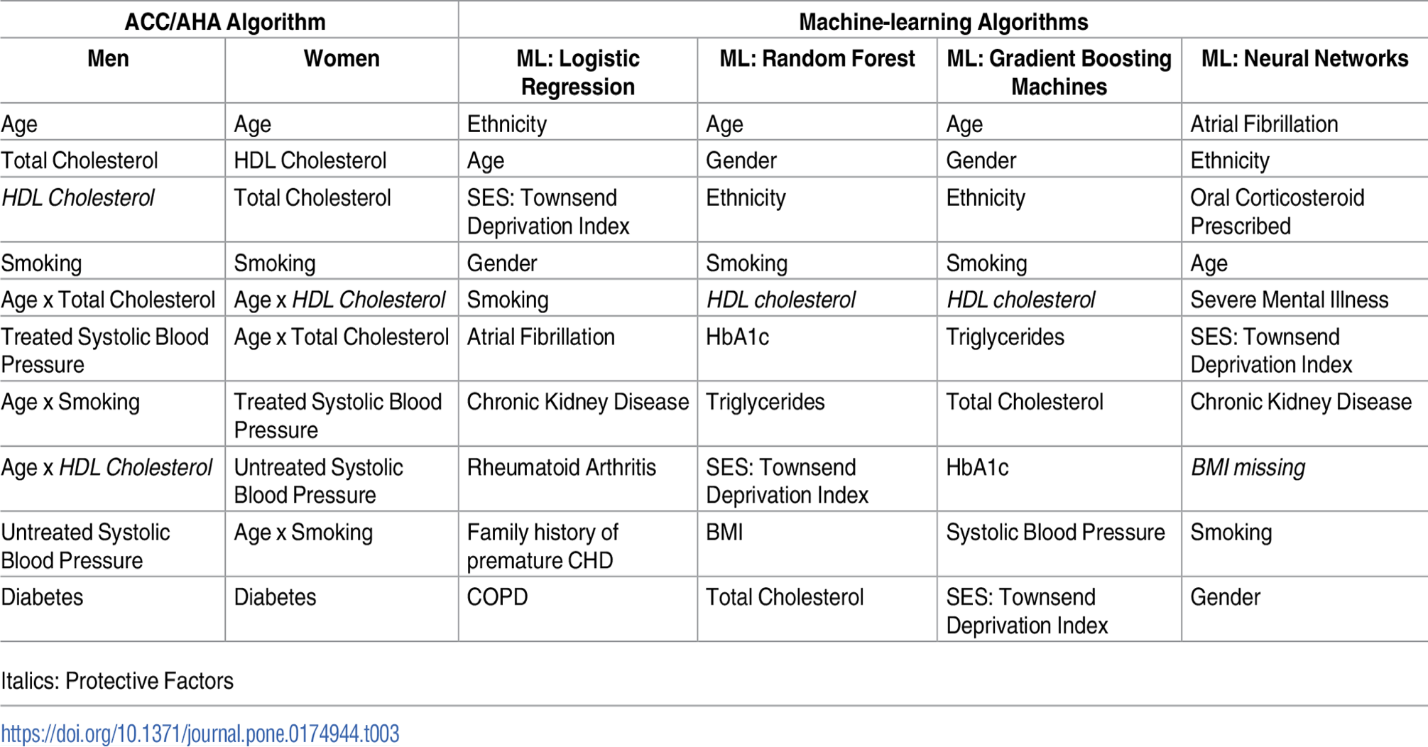Table AP1. Top 10 risk factor variables for cardiovascular disease algorithms listed in descending order of coefficient effect size. Algorithms above were derived from training cohort of 295,267 patients. S.F. Weng, J. Reps, J. Kai, J.M. Garibaldi, N. Qureshi. Can machine-learning improve cardiovascular risk prediction using routine clinical data? PLOS ONE 12(4) e0174944 (2017).

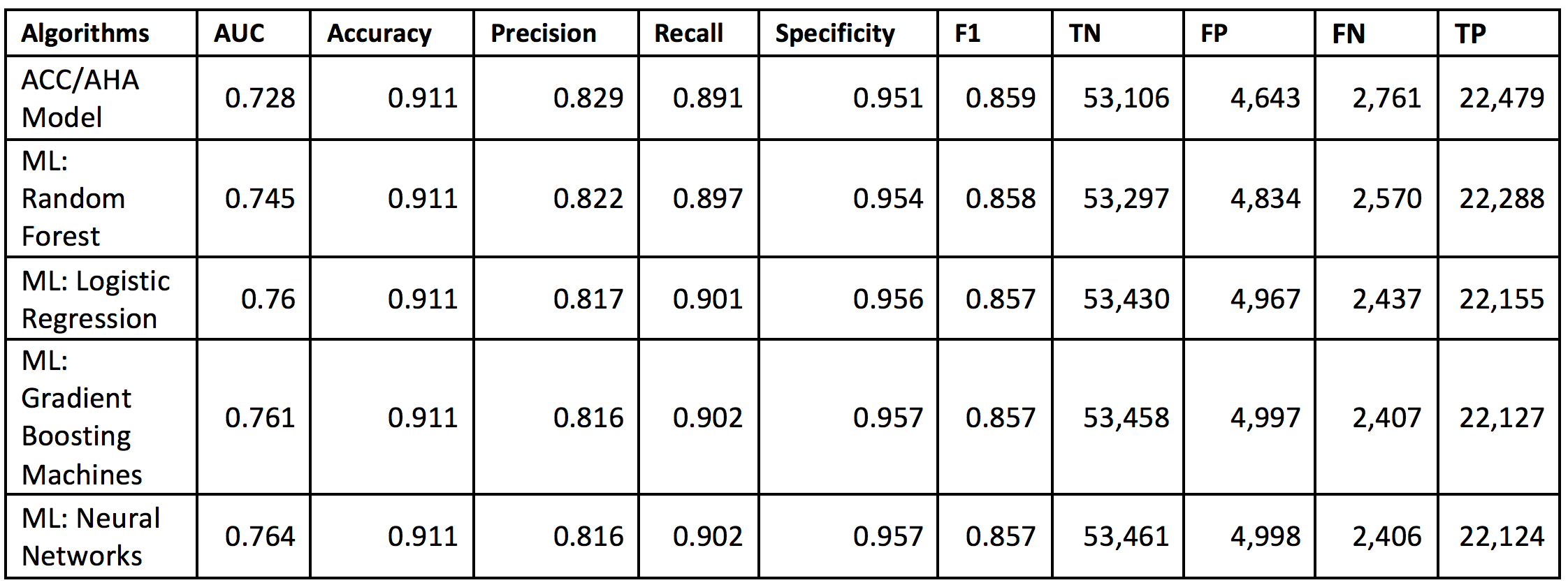Table AP2. Performance of the machine-learning (ML) algorithms predicting 10-year cardiovascular disease (CVD) risk derived from applying training algorithms on the validation cohort of 82,989 patients. S.F. Weng, J. Reps, J. Kai, J.M. Garibaldi, N. Qureshi. Can machine learning improve cardiovascular risk prediction using routine clinical data? PLOS ONE 12(4) e0174944 (2017).

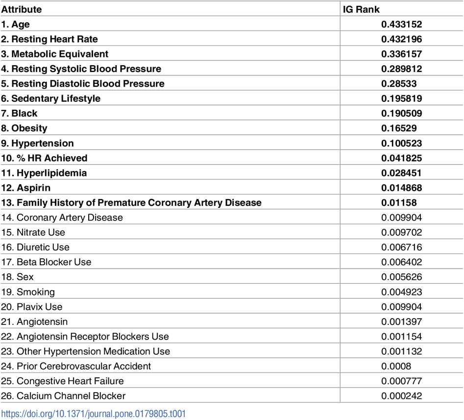Table AP3. Importance Ranking of diabetes predictor features based on their Information Gain (IG) according to M. Alghamdi, M. Al-Mallah, S. Keteyian, C. Brawner, J. Ehrman, et al., Predicting diabetes mellitus using SMOTE and ensemble machine learning approach: The Henry Ford Exercise Testing (FIT) project, PLOS ONE 12(7) e0179805 (2017).

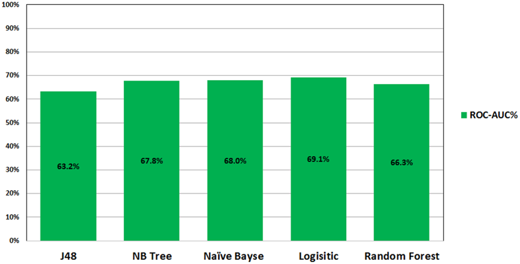Figure AP1. ROC performance of classification models on the imbalance datasets analyzed in the study by M. Alghamdi, M. Al-Mallah, S. Keteyian, C. Brawner, J. Ehrman, et al., Predicting diabetes mellitus using SMOTE and ensemble machine learning approach: The Henry Ford Exercise Testing (FIT) project, PLOS ONE 12(7) e0179805 (2017).

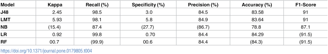Table AP3. Evaluation of the performance of classification models on imbalance dataset, by M. Alghamdi, M. Al-Mallah, S. Keteyian, C. Brawner, J. Ehrman, et al., Predicting diabetes mellitus using SMOTE and ensemble machine learning approach: The Henry Ford Exercise Testing (FIT) project, PLOS ONE 12(7) e0179805 (2017).

Appendix 2: Data pre-processing and feature scaling¶

Questionnaire Data¶

Pre-processing demographics data (DEMO_H.XPT) Resultant features: ['AGE','INCOME_LEVEL', 'ETHNICITY_Black', 'ETHNICITY_Hispanic', 'ETHNICITY_White']

• We restricted the AGE feature column to include only records where respondent's age is between 18 and 65.

• Data imputation was done on the INCOME LEVEL feature by replacing missing values with mean income.

• Re-encoding was done to reorder income level in increasing order.
• Re-encoding was done to replace ETHNICITY integer encoding with string values (ETHNICITY White, ETHNICITY Asian, etc.).
• One-hot encoding of final categorical labels GENDER, ETHNICITY

Pre-processing alcohol consumption level data (ALQ_H.XPT) Resultant feature: ['ALCOHOL_NUM']

• Data imputation was done to replace missing values (unknown consumption) with 0 (person doesn't drink).
• Data imputation was done to fill missing values resulting from re-indexing with mean values.

Pre-processing smoking behavior data (SMQ_H.XPT) Resultant feature: ['SMOKING']

• Data imputation was done to replace missing values (unknown consumption) with 0 (person doesn't smoke).
• Data imputation was done to fill any smoking consumption level with 1 (person smokes).

Pre-processing body weight and height data (WHQ_H.XP) Resultant feature: ['BMI']

• The body-mass index (BMI) feature was not present in original datasets. Only Height h and Weight w were available. Body mass index was calculated using a well-known formula to estimate it. We use it the following function

              def bmi(h, w):
                  return np.round((w/h**2) * 703.0, 2)

Pre-processing nutrition and eating behavior data (DBQ_H.XPT) Resultant features: ['NOTHOME_FOOD', 'FAST_FOOD']

• Data imputation was done to replace missing values in original survey answers with mean value of corresponding feature.

• Data transformation was done to convert food consumption rates to percentage values. If x is number of days where person consumed fast food over a n-day period, then the percent is obtained with

              def percent_transform(x,n):
                      return np.round(float(x/n *100.0),2)

• Data imputation was done to fill missing values resulting from re-indexing with mean values.

Pre-processing cholesterol and blood pressure status data (BPQ_H.XPT) Resultant features: ['HYPERTENSION_ONSET', 'HYPERTENSION', 'HIGHCHOL_ONSET', 'HIGHCHOL']

• There were three features in original dataset indicating that a person had hypertension. We combined these features into the feature 'HYPERTENSION' using an OR operand across the feature columns.

• Since 'HYPERTENSION' is an important predictor for CVD and Diabetes, we replaced missing values with zero to avoid biasing.

Pre-processing health insurance data (HIQ_H.XPT) Resultant features: ['INSURANCE']

• Data imputation was done to replace missing values (unknown insurance status) with 0 (person doesn't have insurance).

Pre-processing cardiovascular health status data (CDQ_H.XPT) Resultant features: ['CHEST_DISCOMFORT', 'CHEST_PAIN_30MIN', 'BREATH_SHORTNESS']

• The features in this group are predictors for CVD and Diabetes, we replaced missing values with zero to avoid biasing.

Pre-processing diabetes status data (DIQ_H.XPT) Resultant features: ['FAMILIAL_DIABETES', 'DIAGNOSED_DIABETES', 'DIAGNOSED_PREDIABETES', 'RISK_DIABETES']

• There were three different possible values of DIAGNOSED_DIABETES that indicated diabetes, and other three which indicated negative for diabetes. We set all this values to 1 (positive for diabetes) and 0 (negative for diabetes, respectively)
• All missing values were replaced by zeroes.

Pre-processing miscellaneous continuous variables Resultant features: ['AGE', 'INCOME_LEVEL', 'ALCOHOL_NUM', 'BMI', 'NOTHOME_FOOD', 'FAST_FOOD']

• We applied a log transform (to alleviate skewness) and scaling via sklearn's RobustScaler(), which scales features to same scale using statistics that are robust to outliers. This Scaler removes the median and scales the data according to the quantile range (defaults to IQR: Interquartile Range).

Standard Biochemistry Profile Data¶

Pre-processing blood biochemistry continuous variables (BIOPRO_H.XPT) Resultant features: all features in dataset

• We applied a log transform (to alleviate skewness) and robust scaling via Sklearn's RobustScaler(), which scales features to same scale using statistics that are robust to outliers. This Scaler removes the median and scales the data according to the quantile range (defaults to IQR: Interquartile Range).

Dataframes Merger¶

All processed questionnaire and laboratory dataframes were integrated into a single dataframe nhanes_df. We performed a final check to ensure no missing values nor un-scaled features where present in the dataframe.