Creating a CNN to Classify Dog Breeds
Now that we have functions for detecting humans and dogs in images, we need a way to predict breed from images. In this step, we create a CNN that classifies dog breeds and build the convolutional network from scratch (we cannot use transfer learning yet!).
Our objective is to attain a test accuracy of at least 1%. In Step 5 of this notebook, we use transfer learning to create a CNN that attains greatly improved accuracy.
At this point we should be careful in adding too many trainable layers! More parameters means longer training, which means we are more likely to need a GPU to accelerate the training process.
Keras provides a handy estimate of the time that each epoch is likely to take; we can extrapolate this estimate to figure out how long it will take for the algorithm to train.
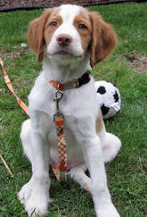
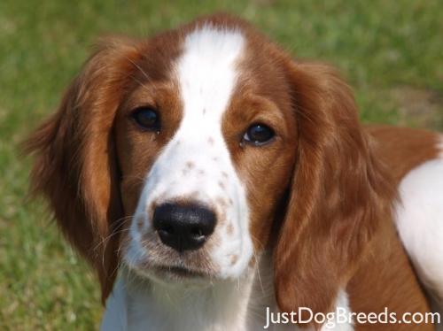
The task of assigning breed to dogs from images is considered exceptionally challenging. To see why, we must consider that even a human would have great difficulty in distinguishing between a Brittany and a Welsh Springer Spaniel.
| Brittany | Welsh Springer Spaniel |
|---|---|
 |
 |
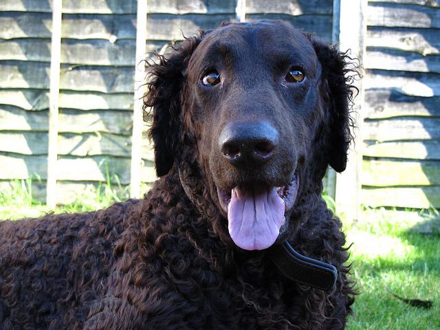
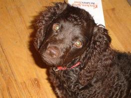
It is not difficult to find other dog breed pairs with minimal inter-class variation (for instance, Curly-Coated Retrievers and American Water Spaniels).
| Curly-Coated Retriever | American Water Spaniel |
|---|---|
 |
 |
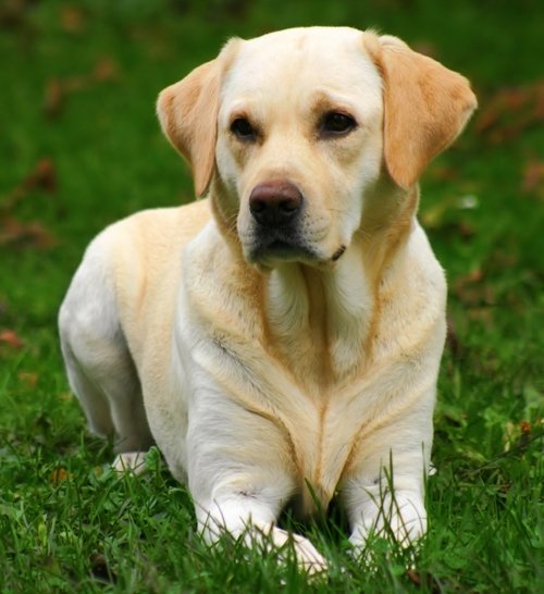
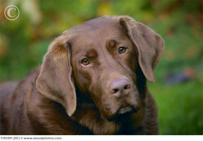
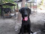
Likewise, recall that labradors come in yellow, chocolate, and black. The computer vision-based algorithm will have to conquer this high intra-class variation to determine how to classify all of these different shades as the same breed.
| Yellow Labrador | Chocolate Labrador | Black Labrador |
|---|---|---|
 |
 |
 |
We also mention that random chance presents an exceptionally low bar: setting aside the fact that the classes are slightly imabalanced, a random guess will provide a correct answer roughly 1 in 133 times, which corresponds to an accuracy of less than 1%.
The practice is far ahead of the theory in deep learning. Experimenting with many different architectures is highly desirable.
Pre-process the Data
We rescale the images by dividing every pixel in every image by 255.
from PIL import ImageFile
ImageFile.LOAD_TRUNCATED_IMAGES = True

# pre-process the data for Keras
train_tensors = paths_to_tensor(train_files).astype('float32')/255
valid_tensors = paths_to_tensor(valid_files).astype('float32')/255
test_tensors = paths_to_tensor(test_files).astype('float32')/255
After executing the previous cell, tensorflow requests about 1.5GB of extra memory. Check the compute process below.
!nvidia-smi
Model Architecture
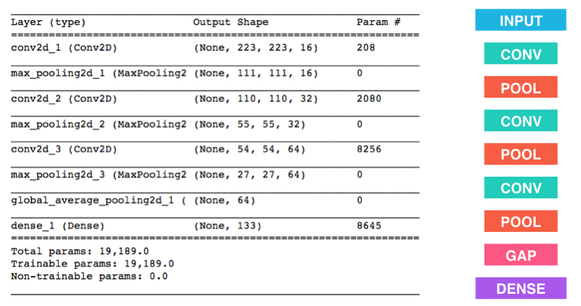
Here I created a CNN to classify a dog breed. At the end the cell block below, I summarized the layers of the model by executing the line:
model.summary()
The following provides an example model that trains relatively fast on CPU and attains >1% test accuracy in 5 epochs:
Below I outline the steps taken to get the final CNN architecture and the reasoning at each step.
Basic steps taken to build and implement a CNN architecture:
Image dataset augmentation.
I augmented both the training and validation datasets by adding random flips and shifts to the original images. This preprocessing benefits the training process and allows the classifier to recognize more variations of the images contained in the validation and testing datasets.
CNN model architecture.
I increased the depth of the CNN originally proposed above by adding two extra convolutional layers, i.e. one additional layer with 128 filters and another one with 256 filters. This change maintains a reasonable total execution time and yields an increase in testing accuracy.
Pre-training analysis.
Before implementing the cnn architecture in the present jupyter notebook I generated a pair of validation curves (using a separate script) to determine the number of epochs to train the model; I did this as a primitive step to fine tune the model. These curves are loaded from png files generated by matplotlib.
Expectations.
I don't expect the CNN architecture proposed above to work well. As given, the CNN is not deep enough to discover and distill enough number of features to appropriately characterize and distinguish dog breeds. However, as shown below, a slight increase in depth can increase the model's accuracy up to 40%, which is still not an acceptable performance metric.
Image augmentation:
#Implements Image Aumentation as done in aind2-cnn jupyter notebook for cifar10
#See https://github.com/udacity/aind2-cnn/blob/master/cifar10-augmentation/

from keras.preprocessing.image import ImageDataGenerator

# create and configure augmented image generator
datagen_train = ImageDataGenerator(
    width_shift_range=0.1,  # randomly shift images horizontally (10% of total width)
    height_shift_range=0.1,  # randomly shift images vertically (10% of total height)
    horizontal_flip=True) # randomly flip images horizontally

# create and configure augmented image generator
datagen_valid = ImageDataGenerator(
    width_shift_range=0.1,  # randomly shift images horizontally (10% of total width)
    height_shift_range=0.1,  # randomly shift images vertically (10% of total height)
    horizontal_flip=True) # randomly flip images horizontally

# fit augmented image generator on data
datagen_train.fit(train_tensors)
datagen_valid.fit(valid_tensors)
CNN Architecture Model:
from keras.layers import Conv2D, MaxPooling2D, GlobalAveragePooling2D
from keras.layers import Dropout, Flatten, Dense
from keras.models import Sequential

model = Sequential()

model.add(Conv2D(filters=16, kernel_size=2, padding='same', activation='relu',
                        input_shape=(224, 224, 3)))
model.add(MaxPooling2D(pool_size=2))
model.add(Conv2D(filters=32, kernel_size=2, padding='same', activation='relu'))
model.add(MaxPooling2D(pool_size=2))
model.add(Conv2D(filters=64, kernel_size=2, padding='same', activation='relu'))
model.add(MaxPooling2D(pool_size=2))
model.add(Conv2D(filters=128, kernel_size=2, padding='same', activation='relu'))
model.add(MaxPooling2D(pool_size=2))
model.add(Conv2D(filters=256, kernel_size=2, padding='same', activation='relu'))
model.add(MaxPooling2D(pool_size=2))
model.add(GlobalAveragePooling2D())
model.add(Dense(133, activation='softmax'))

model.summary()
Compile the Model
model.compile(optimizer='rmsprop', loss='categorical_crossentropy', metrics=['accuracy'])
Training the Model
In the following cell we train the model and use checkpointing to save the model that attains the best validation loss.
We can augment the training data augment the training data, but this is not a requirement.
Pre-training analysis:
show_image('val_curves/scratch_val_curves.png')

The figure above shows plots of the model accuracy and loss function v.s. number epochs for the training and validation sets respectively. The run was implemented in a separate script using a total of 300 epochs and a batch size of 20 samples. The validation loss decays in-between 1 and 100 epochs with significant gains in accuracy. The model shows signs of overfitting when using more than 100 epochs, as the validation loss reverts to an increasing behavior. This suggest using a maximum 100 epochs for model training.
#@Juan E. Rolon
#I added a couple of modifications to allow for measuring the training time
#extract the model fitting history from the checkpointer object. We can use the history
#to monitor the accuracy and loss function during the validation process and save the
#performance metrics to a csv file and generate validation curves plots.

import time
from keras.callbacks import ModelCheckpoint

#specify number of epochs and batch_size
epochs = 100
batch_size = 20

#create checkpointer object to store the model weights
checkpointer = ModelCheckpoint(filepath='saved_models/weights.best.from_scratch.hdf5',
                               verbose=1, save_best_only=True)

init_train_time = time.time()
# Set to True to fit the model to the non-augmented datasets
if False:
    h_scratch = model.fit(train_tensors, train_targets,
              validation_data=(valid_tensors, valid_targets),
              epochs=epochs, batch_size=batch_size, callbacks=[checkpointer], verbose=1)

# Set to True to fit the model to the augmented datasets
if True:
    h_scratch = model.fit_generator(datagen_train.flow(train_tensors, train_targets, batch_size=batch_size),
                        steps_per_epoch=train_tensors.shape[0] // batch_size,
                        epochs=epochs, verbose=1, callbacks=[checkpointer],
                        validation_data=datagen_valid.flow(valid_tensors, valid_targets, batch_size=batch_size),
                        validation_steps=valid_tensors.shape[0] // batch_size)

end_train_time = time.time()
tot_train_time = end_train_time-init_train_time
print("Training time = {0:.3f} minutes ".format(round(tot_train_time/60.0, 3)))
Save checkpoints and generate performance metrics plots:
#@Juan E. Rolon
#Added this function to save performance metrics to csv file and generate corresponding
#plots. It receives the checkpointe history object and a desired filename without
#file extensions. It outputs plots and stores as .csv and .png file respectively.

import pandas as pd

def plotSave_pf_metrics(h, filename):

    #Save history to CSV file
    history_data = pd.DataFrame(h_scratch.history)
    history_data.to_csv(filename + '.csv')

    plt.figure(1, figsize=(10, 4))

    plt.subplot(1,2,1)
    # summarize history for accuracy
    plt.plot(h.history['acc'],color='b')
    plt.plot(h.history['val_acc'],color='k')
    plt.title('Model accuracy')
    plt.ylabel('Accuracy')
    plt.xlabel('Epoch')
    plt.legend(['Train', 'Validation'], loc='upper left')


    plt.subplot(1,2,2)
    # summarize history for loss
    plt.plot(h.history['loss'])
    plt.plot(h.history['val_loss'])
    plt.title('Model loss')
    plt.ylabel('Loss')
    plt.xlabel('Epoch')
    plt.legend(['Train', 'Validation'], loc='upper left')

    #Save and show training and validation performance metrics plots
    plt.savefig(filename + '.png', dpi=300, orientation='landscape')
    plt.show()
plotSave_pf_metrics(h_scratch, 'scratch_cnn_pf_metrics')

Load the Model with the Best Validation Loss
model.load_weights('saved_models/weights.best.from_scratch.hdf5')
Testing the Model
In the cell below we evaluate the model on the test dataset of dog images and attain and accuracy of 40%.
# get index of predicted dog breed for each image in test set
dog_breed_predictions = [np.argmax(model.predict(np.expand_dims(tensor, axis=0))) for tensor in test_tensors]

# report test accuracy
test_accuracy = 100*np.sum(np.array(dog_breed_predictions)==np.argmax(test_targets, axis=1))/len(dog_breed_predictions)
print('Test accuracy: %.4f%%' % test_accuracy)